Distributed Timeserving Routing Policy with Congestion Diversity (D-ORCD)
Info: 11849 words (47 pages) Dissertation
Published: 2nd Feb 2022
CHAPTER 1: LITERATURE SURVEY
1.1 PURPOSE OF THE SYSTEM
The main contribution of this Project is to supply a distributed timeserving routing policy with congestion diversity (D-ORCD), the congestion info is integrated with the distributed shortest path computations.
1.2 EXISTING SYSTEM
The opportunist routing schemes will probably cause severe congestion and boundless delay. In distinction, it’s notable that associate degree opportunist variant of backpressure, diversity backpressure routing (DIVBAR) ensures finite expected total backlog for all stabilizable arrival rates. to make sure outturn optimality (bounded expected total backlog for all stabilizable arrival rates), backpressure-based algorithms do one thing terribly different: instead of victimisation any metric of closeness (or cost) to the destination, they opt for the receiver with the most important positive differential backlog (routing responsibility is preserved by the transmitter if no such receiver exists).
1.2.1 DISADVANTAGES OF EXISTING SYSTEM
The existing property of ignoring the value to the destination, however, becomes the nemesis of this approach, resulting in poor delay performance in low to moderate traffic.
Other existing demonstrably output optimum routing policies distribute the traffic regionally during a manner almost like DIVBAR and therefore, end in massive delay.
1.3 PROPOSED SYSTEM
The main contribution of this paper is to produce a distributed timeserving routing policy with congestion diversity (D-ORCD) below that, rather than a straightforward addition employed in E-DIVBAR, the congestion info is integrated with the distributed shortest path computations.
A comprehensive investigation of the performance of D-ORCD is provided in 2 directions:
We give careful simulation study of delay performance of D-ORCD. we have a tendency to additionally tackle a number of the system-level problems determined in realistic settings via careful simulations.
In addition to the simulation studies, we have a tendency to prove that D-ORCD is outturn best once there’s one destination (single commodity) and also the network operates in stationary regime. whereas characterizing delay performance is commonly not analytically tractable, several variants of backpressure algorithmic program square measure glorious to attain outturn optimality.
1.3.1 BACKGROUND THEORY
OPPORTUNISTIC routing for multi-hop wireless circumstantial networks has long been projected to beat the deficiencies of standard routing. expedient routing mitigates the impact of poor wireless links by exploiting the published nature of wireless transmissions and therefore the path diversity. a lot of exactly, the expedient routing choices square measure created in a web manner by selecting subsequent relay supported the particular transmission outcomes also as a rank ordering of neighboring nodes.
The authors in provided a Andre Markoff call notional formulation for expedient routing and a unified framework for several versions of expedient routing, with the variations owing to the authors’ decisions of prices. particularly, it’s shown that for any packet, the best routing call, within the sense of minimum price or hop-count, is to pick out subsequent relay node supported associate index. This index is adequate the expected price or hop-count of relaying the packet on the smallest amount pricey or the shortest possible path to the destination.
When multiple streams of packets square measure to traverse the network, however, it would be fascinating to route some packets on longer or a lot of pricey methods, if these methods eventually result in links that square measure less engorged. The expedient routing schemes will probably cause severe congestion and boundless delay. In distinction, it’s famed that associate expedient variant of backpressure, diversity backpressure routing (DIVBAR) ensures delimited expected total backlog for all stabilizable arrival rates. To make sure turnout optimality (bounded expected total backlog for all stabilizable arrival rates), backpressure-based algorithms we will do one thing terribly different: instead of mistreatment any metric of closeness (or cost) to the destination, they select the receiver with the most important positive differential backlog (routing responsibility is maintained by the transmitter if no such receiver exists).
This terribly property of ignoring the price to the destination, however, becomes the scourge of this approach, resulting in poor delay performance in low to moderate traffic. different existing demonstrably turnout best routing policies distribute the traffic domestically during a manner just like DIVBAR and thus, lead to massive delay. Recognizing the shortcomings of the 2 approaches, researchers have begun to propose solutions that mix parts of shortest path and backpressure computations, E-DIVBAR is proposed: once selecting subsequent relay among the set of potential forwarders, E-DIVBAR considers the add of the differential backlog and therefore the expected hop-count to the destination (also called ETX). However, E-DIVBAR doesn’t essentially lead to a more robust delay performance than DIVBAR. the most contribution of this paper is to produce a distributed expedient routing policy with congestion diversity (D-ORCD) beneath that, rather than a straightforward addition employed in E-DIVBAR, the congestion data is integrated with the distributed shortest path computations.
A comprehensive investigation of the performance of D-ORCD is provided in 2 directions:
1. We offer elaborate simulation study of delay performance of D-ORCD. we tend to additionally tackle a number of the system-level problems ascertained in realistic settings via elaborate NS2 simulations. we tend to show that D-ORCD exhibits higher delay performance than progressive routing policies with similar complexness, namely, ExOR, DIVBAR, and E-DIVBAR. we tend to additionally show that the relative performance improvement over existing solutions, in general, depends on the topology however is usually important in apply, wherever dead centrosymmetric network preparation and traffic conditions square measure uncommon.
2. Additionally to the simulation studies, we tend to prove that D-ORCD is turnout best once there’s one destination (single commodity) and therefore the network operates in stationary regime. whereas characterizing delay performance is usually not analytically tractable, several variants of backpressure rule square measure famed to attain turnout optimality. we tend to show that an identical analytic guarantee is obtained relating to the turnout optimality of D-ORCD. particularly, we tend to prove the turnout optimality of D-ORCD by watching the convergence of D-ORCD to a centralized version of the rule.
The optimality of the centralized resolution is established via a category of Lyapunov functions projected. Before we tend to shut, we tend to emphasize that a number of the ideas behind the look of D-ORCD have additionally been used as guiding principles in several routing solutions. during this work, however, we’ve chosen to focus our comparative analysis on the subsequent solutions in literature that have similar overhead, complexity, and sensible structure: ExOR, DIVBAR, and E-DIVBAR. still, for the sake of completeness, we tend to detail the similarity and variations between our work. A changed turnout best backpressure policy, LIFO-Backpressure, is projected mistreatment inventory accounting discipline at layer a pair of.
Authors propose a changed version of backpressure that uses the shortest path data to attenuate the typical variety of hops per packet delivery whereas keeping the queues stable. Neither of those approaches lend themselves to sensible implementations: It uses associate atypical inventory accounting computer hardware leading to important rearrangement of packets, which needs maintaining sizable amount of virtual queues at every node increasing implementation complexness. moreover, whereas LIFO-Backpressure policy guarantees stability with nominal queue-length variations, realistic burst traffic in massive multi-hop wireless networks could lead to queue-length variations and unnecessarily high delay.
The authors think about a flow-level model of the network and propose a routing policy observed as min-backlogged-path routing, beneath that the flows square measure routed on the methods with minimum total backlog. compared, D-ORCD is viewed as a packet-based version of the min-backlogged-path routing while not a necessity for the enumeration of methods across the network and/or pricey computations of total backlog on methods.
1.3.2 ADVANTAGES OF PROPOSED SYSTEM
We show that D-ORCD exhibits higher delay performance than progressive routing policies with similar complexness, namely, ExOR, DIVBAR, and E-DIVBAR. We tend to conjointly show that the relative performance improvement over existing solutions, in general, depends on the configuration however is commonly vital in apply, wherever absolutely cruciform network readying and traffic conditions are uncommon.
We show that an analogous analytic guarantee may be obtained relating to the output optimality of D-ORCD. Above all, we tend to prove the output optimality of D-ORCD by viewing the convergence of D-ORCD to a centralized version of the formula. The optimality of the centralized answer is established via a category of Lyapunov functions planned.
CHAPTER 2: SYSTEM REQUIREMENTS
2.1 HARDWARE REQUIREMENTS
- System: Pentium IV 2.4 GHz.
- Hard Disk: 40 GB.
- Floppy Drive: 1.44 Mb.
- Monitor: 15 VGA Colour.
- Mouse: Logitech.
- Ram: 512 Mb.
2.2 SOFTWARE REQUIREMENTS
- Operating system: – Windows XP/7/8/10.
- Coding Language: C, C++
- IDE: NS2 SIMULATOR
CHAPTER 3: SYSTEM DESIGN
3.1 DISTRIBUTED OPPORTUNISTIC ROUTING WITH CONGESTION DIVERSITY (DORCD)
The implementation of D-ORCD, analogous to any timeserving routing theme, involves the choice of a relay node among the candidate set of nodes that have received and acknowledged a packet with success. one in all the most important challenges within the implementation of Associate in Nursing timeserving routing algorithmic program, in general, and D-ORCD particularly, is that the style of compatible acknowledgement mechanism at the mackintosh layer.
The transmission at any node is completed in keeping with CSMA/CA mechanisms. Specially, before any transmission, transmitter performs channel sensing and starts transmission when the rear off counter is decremented to zero. for every neighbor node, the transmitter node then reserves a virtual slot of period, wherever is that the period of the acknowledgement packet and is that the period of Short put down Frame area (SIFS).
Transmitter then piggy-backs a priority ordering of nodes with every information packet transmitted. The priority ordering determines the virtual slot during which the candidate nodes transmit their acknowledgement. Nodes within the set that have with success received the packet then transmit acknowledgement packets consecutive within the order determined by the transmitter node. when a waiting time of throughout that every node within the set has had an opportunity to send Associate in Nursing ACK, node transmits a Forwarding management packet (FO). The field-grade officer packets contain the identity of consecutive forwarder, which can be node itself (i.e., node retains the packet) or any node.
If expires and no field-grade officer packet is received (FO packet reception is unsuccessful), then the corresponding candidate nodes drop the received information packet. If transmitter doesn’t receive any acknowledgement, it retransmits the packet. the rear off window is doubled when each retransmission. what is more, the packet is born if the hear limit (set to7) is reached.
D-ORCD may be a routing policy with improved delay performance over existing timeserving routing policies. during this section, we tend to describe the tenet and the planning of timeserving Routing with Congestion Diversity (D-ORCD). we tend to propose a time-varying distance vector, that permits the network to route packets through a neighbor with the smallest amount calculable delivery time.
D-ORCD opportunistically routes a packet victimization 3 stages of:
(a) transmission,
(b) acknowledgment, and
(c) relaying.
Throughout the transmission stage, a node transmits a packet. throughout the acknowledgment stage, every node that has with success received the transmitted packet, sends Associate in Nursing acknowledgment (ACK) to the transmitter node. D-ORCD then takes routing selections supported a congestion-aware distance vector metric, named because the congestion live. additional specifically, throughout the relaying stage, the relaying responsibility of the packet is shifted to a node with the smallest amount congestion live among those that have received the packet.
The congestion live of a node related to a given destination provides Associate in Nursing estimate of the simplest doable exhausting time of a packet inbound at that node till it reaches destination. every node is accountable to update its congestion live and transmit this data to its neighbors. Next, we tend to detail D-ORCD style and therefore the computations performed at every node to update the congestion live.
3.2 D-ORCD DESIGN
We take into account a network of D nodes labeled by = f1; : : : ;Dg. Let FTO be the likelihood that the packet transmitted by node i is with success received by node j. Node j is claimed to be approachable by node i, if FTO > zero. The set of all nodes within the network that square measure approachable by node i is named as neighborhood of node i and is denoted by N(i). D-ORCD depends on a routing table at every node to see future best hop. The routing table at node i consists of an inventory of neighbors N(i) and a structure consisting of calculable congestion live for all neighbors in N(i) related to totally different destinations.
The routing table acts as a storage and call part at the routing layer. The routing table is updated employing a “virtual routing table” at the top of each “computational cycle”: associate interval Tc units of your time. To update virtual routing table, throughout the progression of the computation cycle the nodes exchange and cipher the temporary congestion measures. The temporary congestion measures square measure computed in a very fashion kind of like a distributed random routing computation of [4] victimization the backlog info at the start of the computation cycle. we tend to conceive this in terms of a virtual routing table change and maintaining these temporary congestion measures. we tend to assume that every node encompasses a common world time to confirm that the nodes update the routing table roughly at an equivalent time. we tend to denote the temporary congestion live related to node i two at time t and destinatifon d two as:
V d i (t). every node i computes V di (t) supported congestion measures ~ V (i;d)
k (t) obtained via periodic communication with its neighbours k two N(i) and also the queue backlog at the beginning of the computation cycle. D-ORCD stores these temporary congestion measures fV di (t)gd2 and f ~ V (i;d) k (t)gd2;k2N(i) within the virtual routing table. a lot of exactly, node i sporadically cipher its own congestion live and afterwards advertises it to its neighbors victimization management packets at intervals of Ts nine Tc seconds. Finally the particular routing table is updated using the entries within the virtual routing table when each Tc seconds. The sequence of operations performed by D-ORCD .Meanwhile, for routing choices, node i uses the entries within the actual routing routing table (computed throughout the lastcomputation cycle). Let T(t) = maxnfnTc : nTc nine t; n two Zg be the ending time of the newest computation cycle. Then nodei stores ~ V (i;d)k (T(t)) within the actual routing table and selects future best hop K(i;d) D ORCD to attenuate the packet’s debilitating time.
CHAPTER 4: TECHNOLOGIES FOR THIS SYSTEM
4.1 NS-2 SIMULATOR
NS2 is associate degree ASCII text file simulation tool that runs on UNIX system. it’s a discreet event machine targeted at networking analysis and provides substantial support for simulation of routing, multicast protocols and science protocols, like UDP, TCP, RTP and SRM over wired and wireless (local and satellite) networks. it’s several benefits that build it a great tool, like support for multiple protocols and therefore the capability of diagrammatically description network traffic. In addition, NS2 supports many algorithms in routing and queuing. square network|LAN|computer network} routing and broadcasts are a part of routing algorithms. Queuing algorithms embody truthful queuing, deficit round-robin and first in first out. NS2 started as a variant of the important network machine in 1989 (see Resources). REAL could be a network machine originally meant for learning the dynamic behavior of flow and congestion management schemes in packet-switched information networks.
Currently NS2 development by VINT cluster is supported through Defense Advanced analysis comes Agency (DARPA) with Albizia saman and thru NSF with CONSER, each unitedly with alternative researchers together with ACIRI (see Resources). NS2 is accessible on many platforms like FreeBSD, Linux, SunOS and Solaris. NS2 conjointly builds and runs underneath Windows.
Simple eventualities ought to run on any cheap machine; but, terribly massive eventualities enjoy massive amounts of memory. In addition, NS2 needs the subsequent packages to run: Tcl unharness eight.3.2, Tk unharness eight.3.2, OTcl unharness one.0a7 and TclCL unharness one.0b11.4.2
4.2 BASIC ARCHITECTURE
NS2 consists of two key languages: C++ and Object-oriented Tool Command Language (OTcl). While the C++ defines the internal mechanism (i.e., a backend) of the simulation objects, the OTcl sets up simulation by assembling and configuring the objects as well as scheduling discrete events. The C++ and the OTcl are linked together using TclCL.
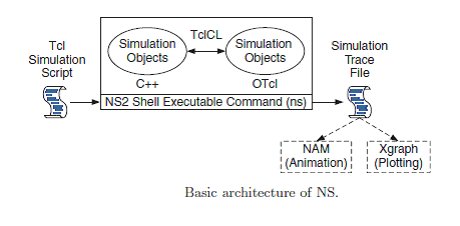
FIG 4.2.1: ARCHITECTURE OF NS2
4.3 TOOLS FOR GENERATING TCL SCRIPTS IN NS-2
Tcl scripts are wide employed in NS-2 simulation tool. Tcl scripts wont to be established a wired or wireless communication network, then run these scripts via the NS-2 for obtaining the simulation results. Several tools are accessible to style networks and generate TCL scripts a number of them are mentioned below
I. NS2 state of affairs Generator (NSG):
It is a java based mostly tool that may run on any platform and may generate TCL scripts for wired and Wireless eventualities for NS2.Main options of NSG are:
1. Making Wired and wireless nodes by drag and drop.
2. Making Simplex and Duplex links for wired network.
3. Making Grid, Random and Chain topologies.
4. Making communications protocol and UDP agents. Conjointly supports communications protocol
5. Tahoe, TCP Reno, communications protocol New-Reno and communications protocol Vegas.
6. Supports spontaneous routing protocols like DSDV,
7. AODV, DSR and TORA.
8. Supports FTP and cosmic microwave background applications.
9. Supports node quality.
10. Setting the packet size, begin time of simulation, end
11. Time of simulation, transmission vary and interference
12. Home in case of wireless networks, etc.
13. Setting different network parameters like information measure, etc for wireless eventualities
II. Visual Network machine (VNS):
This tool is focused on capabilities of NSG. It conjointly provides support to Differentiated Services (DiffServ) eventualities and easy and intuitive set of icons to represent the parts of a network. Some options of VNS ar given below:
1. Adding and configuration of links, agents and traffic sources.
2. Modeling network eventualities with support to multicast.
3. Choice of a dynamic routing protocol.
4. Definition of the simulation output as Associate in Nursing animation and/or graphics.
5. Edition of the Tcl script generated.
6. Saving the outlined simulation state of affairs
III. NS two work bench
Ns Bench makes NS-2 simulation development and analysis quicker and easier for college students and researchers while not losing the flexibleness or quality gained by writing a script. Some options are:
1. Nodes, simplex/duplex links and LANs
2. Agents: communications protocol,UDP, TCPSink, TCP/Fack,TCP/FullTcp, TCP/Newreno, TCP/Reno,TCP/Sack1, TCPSink, TCPSink/Sack1,TCPSink/DelAck,
3. TCPSink/Sack1/DelAck,TCP/Vegas, Null Agent.
4. Applications/Traffic: FTP, Telent, Http/Server,Http/Client, Http/Cache, webtraf, Traffic/CBR,Traffic/Pareto, Traffic/Exponential.
5. Services: Multicast, Packet programing, RED, Diff-Serv.
6. making “Groups” thought to atone for “loops”.
7. state of affairs generator.
8. Link Monitors.
9. Loss Models.
10. Routing Protocols
IV. Network Simulation by Mouse (NSBM)
NSBM, developed in java, may be a graphical tool that’s wont to generate TCL script employing a mouse. Nodes and links will be created with one click. You’ll be able to draw a configuration with multiple nodes with solely a number of mouse clicks. Afterward you click on a button and there’s the TCL code, nearly prepared to be used with the ns.
NSBM employed in order to method the XML configuration knowledge. It should give several functions, that such that solely within the configuration knowledge at run time. As a result of the categories are implementation-specific, categories generated by the binding compiler in one JAXB implementation can in all probability not work with another JAXB implementation. Therefore if you modify to a different JAXB implementation, you must bind the schema with the binding compiler provided by that implementation.
4.4 TRACE FILES GENERATED IN NS-2
NS2 presently supports variety of various forms of trace files. additionally to its own format, NS2 conjointly has the Nam trace format, that contains the required data from the simulation to drive the Nam perceiver. each of those trace formats square measure terribly specific once it involves giving details regarding the events that occur throughout associate NS2 simulation.
Traces and monitors represent the sole support for knowledge assortment in ns-2. Traces record events associated with the generation, enqueueing, forwarding, and dropping of packets. every event corresponds to a line of code characters, that contains data on the event kind and therefore the data keep into the packet
NS-2 provides 3 varieties of formats for wired networks: Tracing, observance and NAM trace file.
I. Tracing: Trace file format is given below:
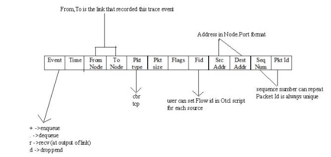
- Operation performed in the simulation
- Simulation time of event occurrence
- Node 1 of what is being traced
- Node 2 of what is being traced
- Packet type
- Packet size
- Flags
- IP flow identifier
- Packet source node address
- Packet destination node address
- Sequence number
- Unique packet identifier
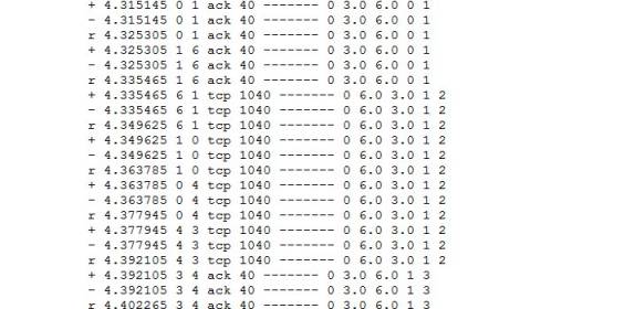
Example of Trace file:
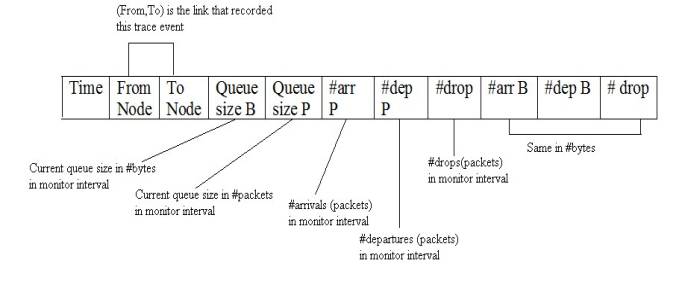
II. Monitoring
Queue monitoring refers to the capability of tracking the dynamics of packets at a queue (or other object). A queue monitor tracks packet arrival/departure/drop statistics, and may optionally compute averages of these values. Monitoring was useful tools to find detail information about queue.
Flow monitor trace format is given below:
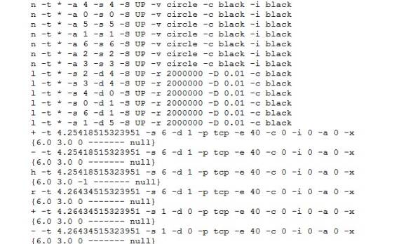
III. NAM trace files which are used by NAM for visualization of ns simulations
The NAM trace file should contain topology information like nodes, links, queues, node connectivity etc as well as packet trace information. A NAM trace file has a basic format to it. Each line is a NAM event. The first character on the line defines the type of event and is followed by several flags to set options on that event. There are 2 sections in that file, static initial configuration events and animation events. All events with -t * in them are configuration events and should be at the beginning of the file.
Example of NAM file is:
CHAPTER 5: SYSTEM DESIGN
5.1 SYSTEM ARCHITECTURE
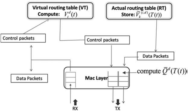
FIG 5.1.1 : SYSTEM ARCHITECTURE
DATA FLOW DIAGRAM
1. The DFD is additionally referred to as as bubble chart. it’s an easy graphical formalism which will be accustomed represent a system in terms of computer file to the system, varied process disbursed on this information, and therefore the output information is generated by this method.
2. the information flow chart (DFD) is one amongst the foremost necessary modeling tools. it’s accustomed model the system elements. These elements square measure the system method, the information employed by the method, associate external entity that interacts with the system and therefore the info flows within the system.
3. DFD shows however the data moves through the system and the way it’s changed by a series of transformations. it’s a graphical technique that depicts info flow and therefore the transformations that square measure applied as information moves from input to output.
4. DFD is additionally referred to as bubble chart. A DFD could also be accustomed represent a system at any level of abstraction. DFD could also be divided into levels that represent increasing info flow and useful detail.
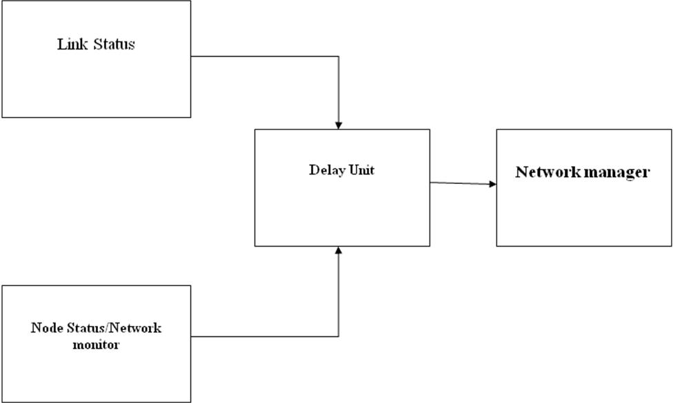
FIG 5.1.2: DATA FLOW DIAGRAM
5.2 UML DIAGRAMS
UML stands for Unified Modeling Language. UML could be a standardized all-purpose modeling language within the field of object-oriented software package engineering. the quality is managed, and was created by, the article Management cluster.
The goal is for UML to become a typical language for making models of object adjusted laptop software package. In its current type UML is comprised of 2 major components: a Meta-model and a notation. within the future, some variety of methodology or method may be more to; or related to, UML.
The Unified Modeling Language could be a commonplace language for specifying, mental image, Constructing and documenting the artifacts of software, further as for business modeling and alternative non-software systems.
The UML represents a set of best engineering practices that have well-tried thriving within the modeling of enormous and sophisticated systems.
The UML could be a vital a part of developing objects adjusted software package and also the software package development method. The UML uses largely graphical notations to specific the planning of software package comes.
GOALS:
The first goals within the style of the UML square measure as follows:
1. Offer users a ready-to-use, communicative visual modeling Language in order that they’ll develop and exchange meaningful models.
2. Offer extendibility and specialization mechanisms to increase the core ideas.
3. Be freelance of specific programming languages and development method.
4. Offer a proper basis for understanding the modeling language.
5. Encourage the expansion of OO tools market.
6. Support higher level development ideas like collaborations, frameworks, patterns and elements.
7. Integrate best practices.
5.2.1 USE CASE DIAGRAM
A use case diagram within the Unified Modeling Language (UML) could be a sort of activity diagram outlined by and created from a Use-case analysis. Its purpose is to gift a graphical summary of the practicality provided by a system in terms of actors, their goals (represented as use cases), and any dependencies between those use cases. the most purpose of a use case diagram is to point out what system functions are performed for which actor. Roles of the actors in the system can be.
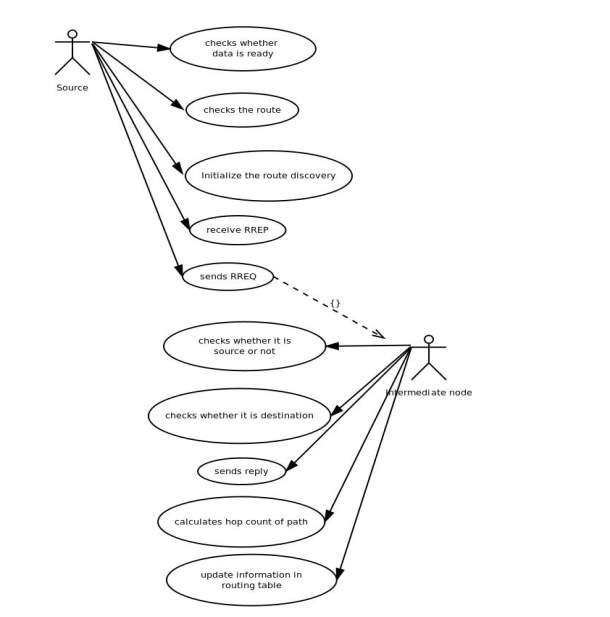
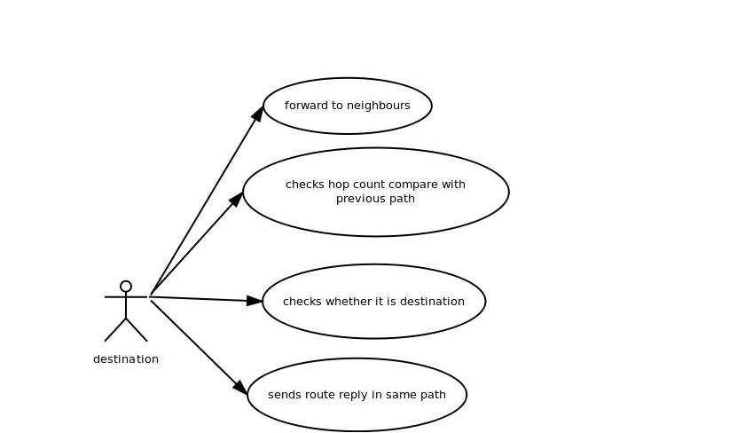
FIG 5.2.1 USE CASE DIAGRAM
5.2.2 CLASS DIAGRAM
In software system engineering, a category diagram within the Unified Modeling Language (UML) may be a sort of static structure diagram that describes the structure of a system by showing the system’s categories, their attributes, operations (or methods), and also the relationships among the categories. It explains that category contains info.
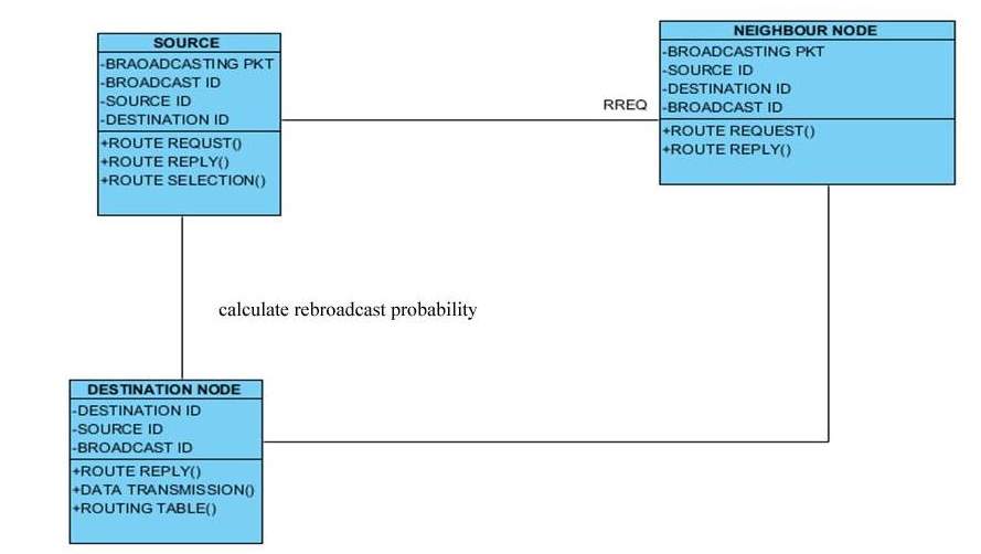
FIG 5.2.2: CLASS DIAGRAM
5.2.3 SEQUENCE DIAGRAM
A sequence diagram in Unified Modeling Language (UML) could be a quite interaction diagram that shows however processes operate with each other and in what order. it’s a construct of a Message Sequence Chart. Sequence diagrams square measure typically known as event diagrams, event situations, and temporal order diagrams.
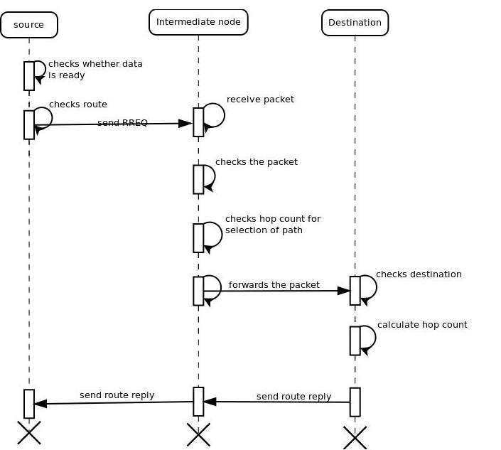
FIG 5.2.3 : SEQUENCE DIAGRAM
5.2.4 ACTIVITY DIAGRAM
Activity diagrams square measure graphical representations of workflows of stepwise activities and actions with support for alternative, iteration and concurrency. within the Unified Modeling Language, activity diagrams are often accustomed describe the business and operational stepwise workflows of parts in an exceedingly system. Associate in Nursing activity diagram shows the flow of management.
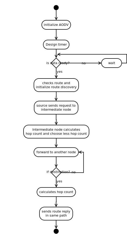
FIG 5.2.4 : ACTIVITY DIAGRAM
CHAPTER 6: SYSTEM IMPLEMENTATION
MODULES:
- System Formation
- Congestion Measure
- Link Quality Estimation Protocol
- Opportunistic Routing With Partial Diversity
MODULES DESCRIPTION:
6.1 SYSTEM FORMATION
In this module, first we develop the System Formation concepts. We consider a network of D nodes labeled by Ω= {1,….,D} . We characterize the behavior of the wireless channel using a probabilistic transmission model. Node is said to be neighbor of node , if there is a positive probability pij that a transmission at node i is received at node . The set of all nodes in the network which are reachable by node is referred to as neighborhood of node.
D-ORCD relies on a routing table at each node to determine the next best hop. The routing table at node consists of a list of neighbors and a structure consisting of estimated congestion measure for all neighbors in associated with different destinations.
The routing table acts as a storage and decision component at the routing layer. The routing table is updated using a “virtual routing table” at the end of every “computation cycle”: an interval of units of time.
To update virtual routing table, during the progression of the computation cycle the nodes exchange and compute the temporary congestion measures.
6.2 CONGESTION MEASURE
In this module, we develop the proposed system by this the system can able to identify the Congestion happened. The Congestion measure values are code and defined in the module.
The congestion measure associated with node for a destination at time is the aggregate sum of the local draining time at node and the draining time from its next hop to the destination. D-ORCD computes the expected congestion measure “down the stream”.
The implementation of D-ORCD, analogous to any opportunistic routing scheme, involves the selection of a relay node among the candidate set of nodes that have received and acknowledged a packet successfully. One of the major challenges in the implementation of an opportunistic routing algorithm, in general, and D-ORCD in particular, is the design of an 802.11 compatible acknowledgement mechanism at the MAC layer.
6.3 LINK QUALITY ESTIMATION PROTOCOL
In this module we develop the Link Quality Estimation Protocol for the proposed system model. D-ORCD computations given by (1) utilize link success probabilities pij for each pair of nodes i,j. We now describe a method to determine the probability of successfully receiving a data packet for each pair of nodes.
Our method consists of two components: active probing and passive probing.
In the active probing, dedicated probe packets are broadcasted periodically to estimate link success probabilities.
In passive probing, the overhearing capability of the wireless medium are utilized. The nodes are configured to promiscuous mode, hence enabling them to hear the packets from neighbors. In passive probing, the MAC layer keeps track of the number of packets received from the neighbors including the retransmissions.
Finally, a weighted average is used to combine the active and passive estimates to determine the link success probabilities. Passive probing does not introduce any additional overhead cost but can be slow, while active probing rate is set independently of the data rate but introduces costly overhead.
6.4 OPPORTUNSTIC ROUTING WITH PARTIAL DIVERSITY
In the module, the opportunistic Routing part is implemented and developed in the proposed system model. The three-way handshake procedure achieves opportunism and receiver diversity gain at the cost of an increased feedback overhead. In particular, it is easy to see that this overhead cost, i.e., the total number of ACKs sent per data packet transmission, increases linearly with the size of the set of potential forwarders. Thus, we consider a modification of D-ORCD in the form of opportunistically routing with partial diversity (PD-ORCD).
This class of routing policies is parametrized by a parameter denoting the maximum number of forwarder nodes: the maximum number of nodes allowed to send acknowledgment per data packet transmission is constrained to be no more than.Such a constraint will sacrifice the diversity gain, and hence the performance of any opportunistic routing policy, in favor of lowering overhead cost.
In order to implement opportunistic routing policies with partial diversity, before the transmission stage occurs, we find the set of “best neighbors” for each node.
CHAPTER 7: SAMPLE CODE
7.1 Main FILE
/* set val(chan) Channel/WirelessChannel ;
set val(prop) Propagation/TwoRayGround ;
set val(netif) Phy/WirelessPhy ;
set val(mac) Mac/802_11 ;
set val(ifq) Queue/DropTail/PriQueue ;
set val(ll) LL ;
set val(ant) Antenna/OmniAntenna ;
set val(ifqlen) 1000 ;
set val(nn) 33 ;
set val(rp) DSR ;
set val(x) 500
set val(y) 500
set ns_ [new Simulator]
set tracefd [open output.tr w]
$ns_ trace-all $tracefd
set namtrace [open mobile_con.nam w]
$ns_ namtrace-all-wireless $namtrace $val(x) $val(y)
set topo [new Topography]
$topo load_flatgrid $val(x) $val(y)
create-god $val(nn)
set chan_1_ [new $val(chan)]
set chan_2_ [new $val(chan)]
$ns_ node-config -adhocRouting $val(rp)
-llType $val(ll)
-macType $val(mac)
-ifqType $val(ifq)
-ifqLen $val(ifqlen)
-antType $val(ant)
-propType $val(prop)
-phyType $val(netif)
-topoInstance $topo
-agentTrace ON
-routerTrace ON
-macTrace ON
-movementTrace ON
-channel $chan_1_
$ns_ node-config channel $chan_2_
set node_(0) [$ns_ node]
set node_(1) [$ns_ node]
set node_(2) [$ns_ node]
set node_(3) [$ns_ node]
set node_(4) [$ns_ node]
set node_(5) [$ns_ node]
set node_(6) [$ns_ node]
set node_(7) [$ns_ node]
set node_(8) [$ns_ node]
set node_(9) [$ns_ node]
set node_(10) [$ns_ node]
set node_(11) [$ns_ node]
set node_(12) [$ns_ node]
set node_(13) [$ns_ node]
set node_(14) [$ns_ node]
set node_(15) [$ns_ node]
set node_(16) [$ns_ node]
set node_(17) [$ns_ node]
set node_(18) [$ns_ node]
set node_(19) [$ns_ node]
set node_(20) [$ns_ node]
set node_(21) [$ns_ node]
set node_(22) [$ns_ node]
set node_(23) [$ns_ node]
set node_(24) [$ns_ node]
set node_(25) [$ns_ node]
set node_(26) [$ns_ node]
set node_(27) [$ns_ node]
set node_(28) [$ns_ node]
set node_(29) [$ns_ node]
set node_(30) [$ns_ node]
set node_(31) [$ns_ node]
set node_(32) [$ns_ node]
for {set i 0} {$i < $val(nn)} {incr i} {
$ns_ initial_node_pos $node_($i) 30
}
$node_(0) set X_ 527.117
$node_(0) set Y_ 125.829
$node_(0) set Z_ 0.0
$node_(1) set X_ 360.446
$node_(1) set Y_ 404.907
$node_(1) set Z_ 0.0
$node_(2) set X_ 335.384
$node_(2) set Y_ 97.629
$node_(2) set Z_ 0.0
$node_(3) set X_ 131.14
$node_(3) set Y_ 402.031
$node_(3) set Z_ 0.0
$node_(4) set X_ 39.969
$node_(4) set Y_ 118.743
$node_(4) set Z_ 0.0
$node_(5) set X_ 85.532
$node_(5) set Y_ 235.008
$node_(5) set Z_ 0.0
$node_(6) set X_ 455.608
$node_(6) set Y_ 92.476
$node_(6) set Z_ 0.0
$node_(7) set X_ 500.482
$node_(7) set Y_ 340.148
$node_(7) set Z_ 0.0
$node_(8) set X_ 287.533
$node_(8) set Y_ 404.116
$node_(8) set Z_ 0.0
$node_(9) set X_ 508.053
$node_(9) set Y_ 420.814
$node_(9) set Z_ 0.0
$node_(10) set X_ 93.3994
$node_(10) set Y_ 318.466
$node_(10) set Z_ 0.0
$node_(11) set X_ 40.189
$node_(11) set Y_ 362.477
$node_(11) set Z_ 0.0
$node_(12) set X_ 259.189
$node_(12) set Y_ 307.477
$node_(12) set Z_ 0.0
$node_(13) set X_ 405.354
$node_(13) set Y_ 251.199
$node_(13) set Z_ 0.0
$node_(14) set X_ 527.035
$node_(14) set Y_ 290.136
$node_(14) set Z_ 0.0
$node_(15) set X_ 127.189
$node_(15) set Y_ 128.477
$node_(15) set Z_ 0.0
$node_(16) set X_ 22.189
$node_(16) set Y_ 251.477
$node_(16) set Z_ 0.0
$node_(17) set X_ 433.416
$node_(17) set Y_ 37.6304
$node_(17) set Z_ 0.0
$node_(18) set X_ 202.189
$node_(18) set Y_ 385.477
$node_(18) set Z_ 0.0
$node_(19) set X_ 421.189
$node_(19) set Y_ 433.477
$node_(19) set Z_ 0.0
$node_(20) set X_ 250.189
$node_(20) set Y_ 445.477
$node_(20) set Z_ 0.0
$node_(21) set X_ 338.138
$node_(21) set Y_ 240.591
$node_(21) set Z_ 0.0
$node_(22) set X_ 327.189
$node_(22) set Y_ 185.477
$node_(22) set Z_ 0.0
$node_(23) set X_ 194.672
$node_(23) set Y_ 87.4259
$node_(23) set Z_ 0.0
$node_(24) set X_ 235.189
$node_(24) set Y_ 131.477
$node_(24) set Z_ 0.0
$node_(25) set X_ 362.013
$node_(25) set Y_ 36.9827
$node_(25) set Z_ 0.0
$node_(26) set X_ 375.189
$node_(26) set Y_ 184.477
$node_(26) set Z_ 0.0
$node_(27) set X_ 20.189
$node_(27) set Y_ 174.477
$node_(27) set Z_ 0.0
$node_(28) set X_ 220.189
$node_(28) set Y_ 184.477
$node_(28) set Z_ 0.0
$node_(29) set X_ 490.189
$node_(29) set Y_ 184.477
$node_(29) set Z_ 0.0
$node_(30) set X_ 125.62
$node_(30) set Y_ 58.74
$node_(30) set Z_ 0.0
$node_(31) set X_ 120.289
$node_(31) set Y_ 472.577
$node_(31) set Z_ 0.0
$node_(32) set X_ 370.289
$node_(32) set Y_ 307.577
$node_(32) set Z_ 0.0
$ns_ at 0 “$node_(0) setdest 290.215 473.559 0.0”
$ns_ at 0 “$node_(1) setdest 448.148 275.592 0.0”
$ns_ at 0 “$node_(2) setdest 254.275 5.02 0.0”
$ns_ at 0 “$node_(3) setdest 113.189 455.723 0.0”
$ns_ at 0 “$node_(4) setdest 258.962 27.64 0.0”
$ns_ at 0 “$node_(5) setdest 451.532 209.008 0.0”
$ns_ at 0 “$node_(6) setdest 157.608 285.576 0.0”
$ns_ at 0 “$node_(7) setdest 317.455 319.148 0.0”
$ns_ at 0 “$node_(8) setdest 90.553 399.116 0.0”
$ns_ at 0 “$node_(9) setdest 409.053 478.814 0.0”
$ns_ at 0 “$node_(10) setdest 290.189 473.477 0.0”
$ns_ at 0 “$node_(11) setdest 193.189 125.477 0.0”
$ns_ at 0 “$node_(12) setdest 330.189 368.477 0.0”
$ns_ at 0 “$node_(13) setdest 448.189 368.477 0.0”
$ns_ at 0 “$node_(14) setdest 295.189 225.477 0.0”
$ns_ at 0 “$node_(15) setdest 377.189 152.477 0.0”
$ns_ at 0 “$node_(16) setdest 77.189 415.477 0.0”
$ns_ at 0 “$node_(17) setdest 276.189 462.477 0.0”
$ns_ at 0 “$node_(18) setdest 300.189 338.477 0.0”
$ns_ at 0 “$node_(19) setdest 39.189 342.477 0.0”
$ns_ at 0 “$node_(20) setdest 478.189 6.477 0.0”
$ns_ at 0 “$node_(21) setdest 44.189 87.477 0.0”
$ns_ at 0 “$node_(22) setdest 485.189 339.477 0.0”
$ns_ at 0 “$node_(23) setdest 159.189 2.477 0.0”
$ns_ at 0 “$node_(24) setdest 411.189 32.477 0.0”
$ns_ at 0 “$node_(25) setdest 470.189 215.477 0.0”
$ns_ at 0 “$node_(26) setdest 325.189 92.477 0.0”
$ns_ at 0 “$node_(27) setdest 125.189 292.477 0.0”
$ns_ at 0 “$node_(28) setdest 425.189 192.477 0.0”
$ns_ at 0 “$node_(29) setdest 225.189 392.477 0.0”
$ns_ at 0 “$node_(30) setdest 125.62 58.74 0.0”
$ns_ at 0 “$node_(31) setdest 120.289 472.577 0.0”
$ns_ at 0 “$node_(32) setdest 370.289 307.577 0.0”
$ns_ at 0.1 “$node_(0) color green”
$ns_ at 0.1 “$node_(1) color green”
$ns_ at 0.1 “$node_(2) color green”
$ns_ at 0.1 “$node_(3) color green”
$ns_ at 0.1 “$node_(4) color green”
$ns_ at 0.1 “$node_(5) color green”
$ns_ at 0.1 “$node_(6) color green”
$ns_ at 0.1 “$node_(7) color green”
$ns_ at 0.1 “$node_(8) color green”
$ns_ at 0.1 “$node_(9) color green”
$ns_ at 0.1 “$node_(10) color green”
$ns_ at 0.1 “$node_(11) color green”
$ns_ at 0.1 “$node_(12) color green”
$ns_ at 0.1 “$node_(13) color green”
$ns_ at 0.1 “$node_(14) color green”
$ns_ at 0.1 “$node_(15) color green”
$ns_ at 0.1 “$node_(16) color green”
$ns_ at 0.1 “$node_(17) color green”
$ns_ at 0.1 “$node_(18) color green”
$ns_ at 0.1 “$node_(19) color green”
$ns_ at 0.1 “$node_(20) color green”
$ns_ at 0.1 “$node_(21) color green”
$ns_ at 0.1 “$node_(22) color green”
$ns_ at 0.1 “$node_(23) color green”
$ns_ at 0.1 “$node_(24) color green”
$ns_ at 0.1 “$node_(25) color green”
$ns_ at 0.1 “$node_(26) color green”
$ns_ at 0.1 “$node_(27) color green”
$ns_ at 0.1 “$node_(28) color green”
$ns_ at 0.1 “$node_(29) color green”
$ns_ at 0.1 “$node_(30) color green”
$ns_ at 0.1 “$node_(31) color green”
$ns_ at 0.1 “$node_(32) color green”
set color_name(1) black
$ns_ at 0.1 “$node_(10) add-mark m0 magenta hexagon”
$ns_ at 0.1 “$node_(10) label Source”
for {set i 0} {$i<30} {incr i} {
set sink($i) [new Agent/LossMonitor]
$ns_ attach-agent $node_($i) $sink($i)
}
#—————————- CBR Traffic Creation ———————–
proc attach-CBR-traffic { node sink pkt int } {
global ns_
set udp [new Agent/UDP]
$ns_ attach-agent $node $udp
#Create a CBR agent and attach it to the node
set cbr [new Application/Traffic/CBR]
$cbr attach-agent $udp
$cbr set packetSize_ $pkt ;#sub packet size
$cbr set interval_ $int
#Attach CBR source to sink;
$ns_ connect $udp $sink
return $cbr
}*/
7.2 Output Trace File ( sample):
/* Sconfig 0.00000 tap: on snoop: rts? on errs? on
Sconfig 0.00000 salvage: on !bd replies? on
Sconfig 0.00000 grat error: on grat reply: on
Sconfig 0.00000 $reply for props: on ring 0 search: on
Sconfig 0.00000 using MOBICACHE
M 0.00000 0 (527.12, 125.83, 0.00), (290.21, 473.56), 0.00
M 0.00000 1 (360.45, 404.91, 0.00), (448.15, 275.59), 0.00
M 0.00000 2 (335.38, 97.63, 0.00), (254.28, 5.02), 0.00
M 0.00000 3 (131.14, 402.03, 0.00), (113.19, 455.72), 0.00
M 0.00000 4 (39.97, 118.74, 0.00), (258.96, 27.64), 0.00
M 0.00000 5 (85.53, 235.01, 0.00), (451.53, 209.01), 0.00
M 0.00000 6 (455.61, 92.48, 0.00), (157.61, 285.58), 0.00
M 0.00000 7 (500.48, 340.15, 0.00), (317.45, 319.15), 0.00
M 0.00000 8 (287.53, 404.12, 0.00), (90.55, 399.12), 0.00
M 0.00000 9 (508.05, 420.81, 0.00), (409.05, 478.81), 0.00
M 0.00000 10 (93.40, 318.47, 0.00), (290.19, 473.48), 0.00
M 0.00000 11 (40.19, 362.48, 0.00), (193.19, 125.48), 0.00
M 0.00000 12 (259.19, 307.48, 0.00), (330.19, 368.48), 0.00
M 0.00000 13 (405.35, 251.20, 0.00), (448.19, 368.48), 0.00
M 0.00000 14 (527.03, 290.14, 0.00), (295.19, 225.48), 0.00
M 0.00000 15 (127.19, 128.48, 0.00), (377.19, 152.48), 0.00
M 0.00000 16 (22.19, 251.48, 0.00), (77.19, 415.48), 0.00
M 0.00000 17 (433.42, 37.63, 0.00), (276.19, 462.48), 0.00
M 0.00000 18 (202.19, 385.48, 0.00), (300.19, 338.48), 0.00
M 0.00000 19 (421.19, 433.48, 0.00), (39.19, 342.48), 0.00
M 0.00000 20 (250.19, 445.48, 0.00), (478.19, 6.48), 0.00
M 0.00000 21 (338.14, 240.59, 0.00), (44.19, 87.48), 0.00
M 0.00000 22 (327.19, 185.48, 0.00), (485.19, 339.48), 0.00
M 0.00000 23 (194.67, 87.43, 0.00), (159.19, 2.48), 0.00
M 0.00000 24 (235.19, 131.48, 0.00), (411.19, 32.48), 0.00
M 0.00000 25 (362.01, 36.98, 0.00), (470.19, 215.48), 0.00
M 0.00000 26 (375.19, 184.48, 0.00), (325.19, 92.48), 0.00
M 0.00000 27 (20.19, 174.48, 0.00), (125.19, 292.48), 0.00
M 0.00000 28 (220.19, 184.48, 0.00), (425.19, 192.48), 0.00
M 0.00000 29 (490.19, 184.48, 0.00), (225.19, 392.48), 0.00
M 0.00000 30 (125.62, 58.74, 0.00), (125.62, 58.74), 0.00
M 0.00000 31 (120.29, 472.58, 0.00), (120.29, 472.58), 0.00
M 0.00000 32 (370.29, 307.58, 0.00), (370.29, 307.58), 0.00
v 0 eval {set sim_annotation {Simulation Begins}}
s 0.100000000 _10_ AGT — 0 tcp 40 [0 0 0 0] ——- [10:1 12:1 32 0] [0 0] 0 0
r 0.100000000 _10_ RTR — 0 tcp 40 [0 0 0 0] ——- [10:1 12:1 32 0] [0 0] 0 0
s 0.100000000 _10_ AGT — 2 tcp 40 [0 0 0 0] ——- [10:2 8:1 32 0] [0 0] 0 0
r 0.100000000 _10_ RTR — 2 tcp 40 [0 0 0 0] ——- [10:2 8:1 32 0] [0 0] 0 0
s 0.100000000 _10_ AGT — 4 tcp 40 [0 0 0 0] ——- [10:3 28:1 32 0] [0 0] 0 0
r 0.100000000 _10_ RTR — 4 tcp 40 [0 0 0 0] ——- [10:3 28:1 32 0] [0 0] 0 0
v 0.10000000000000001 eval {set sim_annotation {Node Formations >> N1 to N20}}
s 0.106153566 _10_ RTR — 3 DSR 32 [0 0 0 0] ——- [10:255 8:255 32 0] 1 [1 2] [0 2 0 0->0] [0 0 0 0->0]
s 0.106288566 _10_ MAC — 3 DSR 90 [0 ffffffff a 800] ——- [10:255 8:255 32 0] 1 [1 2] [0 2 0 0->0] [0 0 0 0->0]
r 0.107008796 _11_ MAC — 3 DSR 32 [0 ffffffff a 800] ——- [10:255 8:255 32 0] 1 [1 2] [0 2 0 0->0] [0 0 0 0->0]
r 0.107008846 _5_ MAC — 3 DSR 32 [0 ffffffff a 800] ——- [10:255 8:255 32 0] 1 [1 2] [0 2 0 0->0] [0 0 0 0->0]
r 0.107008872 _3_ MAC — 3 DSR 32 [0 ffffffff a 800] ——- [10:255 8:255 32 0] 1 [1 2] [0 2 0 0->0] [0 0 0 0->0]
r 0.107008892 _16_ MAC — 3 DSR 32 [0 ffffffff a 800] ——- [10:255 8:255 32 0] 1 [1 2] [0 2 0 0->0] [0 0 0 0->0]
r 0.107008992 _18_ MAC — 3 DSR 32 [0 ffffffff a 800] ——- [10:255 8:255 32 0] 1 [1 2] [0 2 0 0->0] [0 0 0 0->0]
r 0.107009088 _31_ MAC — 3 DSR 32 [0 ffffffff a 800] ——- [10:255 8:255 32 0] 1 [1 2] [0 2 0 0->0] [0 0 0 0->0]
r 0.107009105 _27_ MAC — 3 DSR 32 [0 ffffffff a 800] ——- [10:255 8:255 32 0] 1 [1 2] [0 2 0 0->0] [0 0 0 0->0]
r 0.107009120 _12_ MAC — 3 DSR 32 [0 ffffffff a 800] ——- [10:255 8:255 32 0] 1 [1 2] [0 2 0 0->0] [0 0 0 0->0]
r 0.107009181 _28_ MAC — 3 DSR 32 [0 ffffffff a 800] ——- [10:255 8:255 32 0] 1 [1 2] [0 2 0 0->0] [0 0 0 0->0]
r 0.107009209 _15_ MAC — 3 DSR 32 [0 ffffffff a 800] ——- [10:255 8:255 32 0] 1 [1 2] [0 2 0 0->0] [0 0 0 0->0]
r 0.107009239 _20_ MAC — 3 DSR 32 [0 ffffffff a 800] ——- [10:255 8:255 32 0] 1 [1 2] [0 2 0 0->0] [0 0 0 0->0]
r 0.107009255 _4_ MAC — 3 DSR 32 [0 ffffffff a 800] ——- [10:255 8:255 32 0] 1 [1 2] [0 2 0 0->0] [0 0 0 0->0]
r 0.107009274 _8_ MAC — 3 DSR 32 [0 ffffffff a 800] ——- [10:255 8:255 32 0] 1 [1 2] [0 2 0 0->0] [0 0 0 0->0]
r 0.107009348 _24_ MAC — 3 DSR 32 [0 ffffffff a 800] ——- [10:255 8:255 32 0] 1 [1 2] [0 2 0 0->0] [0 0 0 0->0]
r 0.107033796 _11_ RTR — 3 DSR 32 [0 ffffffff a 800] ——- [10:255 8:255 32 0] 1 [1 2] [0 2 0 0->0] [0 0 0 0->0] */
CHAPTER 8: SCREENSHOTS
8.1: To start Cygwin
In order to start the simulation, the Cygwin command prompt must be used.
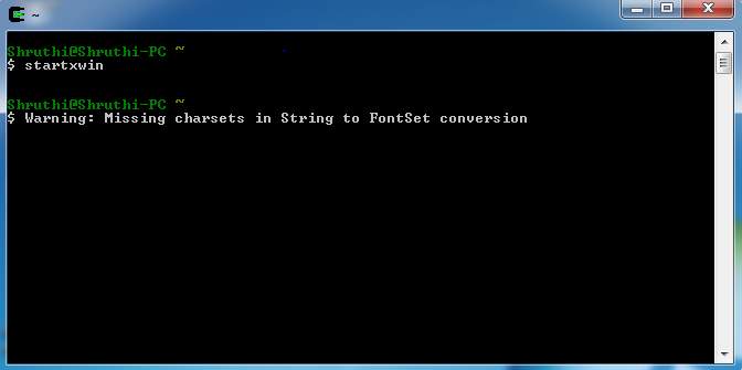
FIG 8.1.1 – STARTING CYGWIN
8.2: After starting Cygwin, the network animator will open and will ask for the location of the fie for which the simulation has to be run.
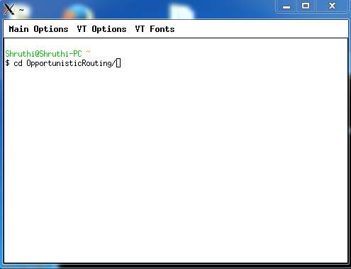
FIG 8.2.1 – NETWORK ANIMATOR
8.3: In order to start the simulation the main file has to be run
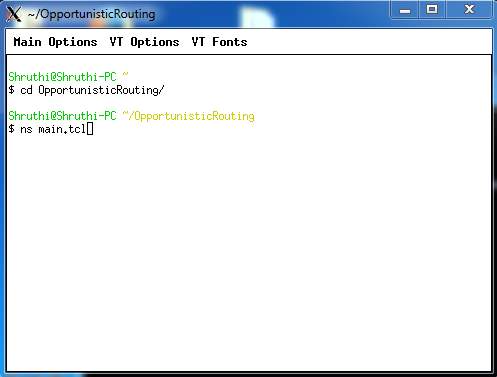
FIG 8.3.1 – TO EXECUTE THE FILE
8.4: The input has to be provided for the file to run accordingly
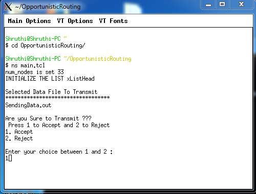
FIG 8.4.1 – TO PROVIDE INPUT
8.5: To enter the transmission size of packet to send in the network.
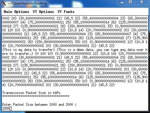
FIG 8.5.1 – TO ENTER TRANSMISSION PACKET SIZE
8.6: To enter individual node strength
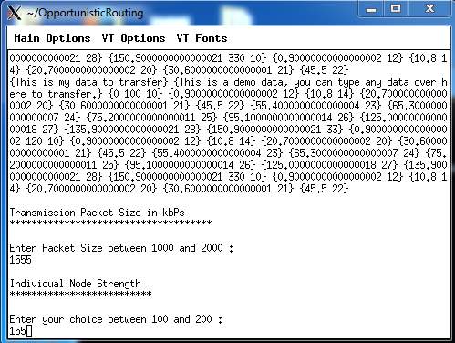
FIG 8.6.1 – ENTER INDIVIDUAL NODE STRENGTH
8.7: To enter packet transmission speed
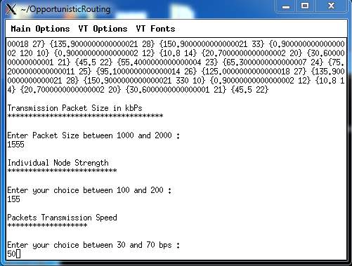
FIG 8.7.1 – PACKET TRANSMISSION SPEED
8.8: To enter average power transmission speed
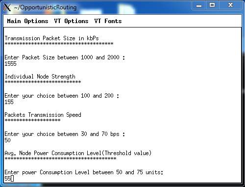
FIG 8.8.1 – AVERAGE POWER TRANSMISSION SPEED
8.9: To enter average time interval
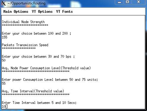
FIG 8.9.1 – AVERAGE TIME INTERVAL
8.10: Simulation starts
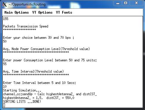
FIG 8.10.1 – SIMULATION BEGINS
8.11: Simulation starts. Adjust the speed of the simulation.
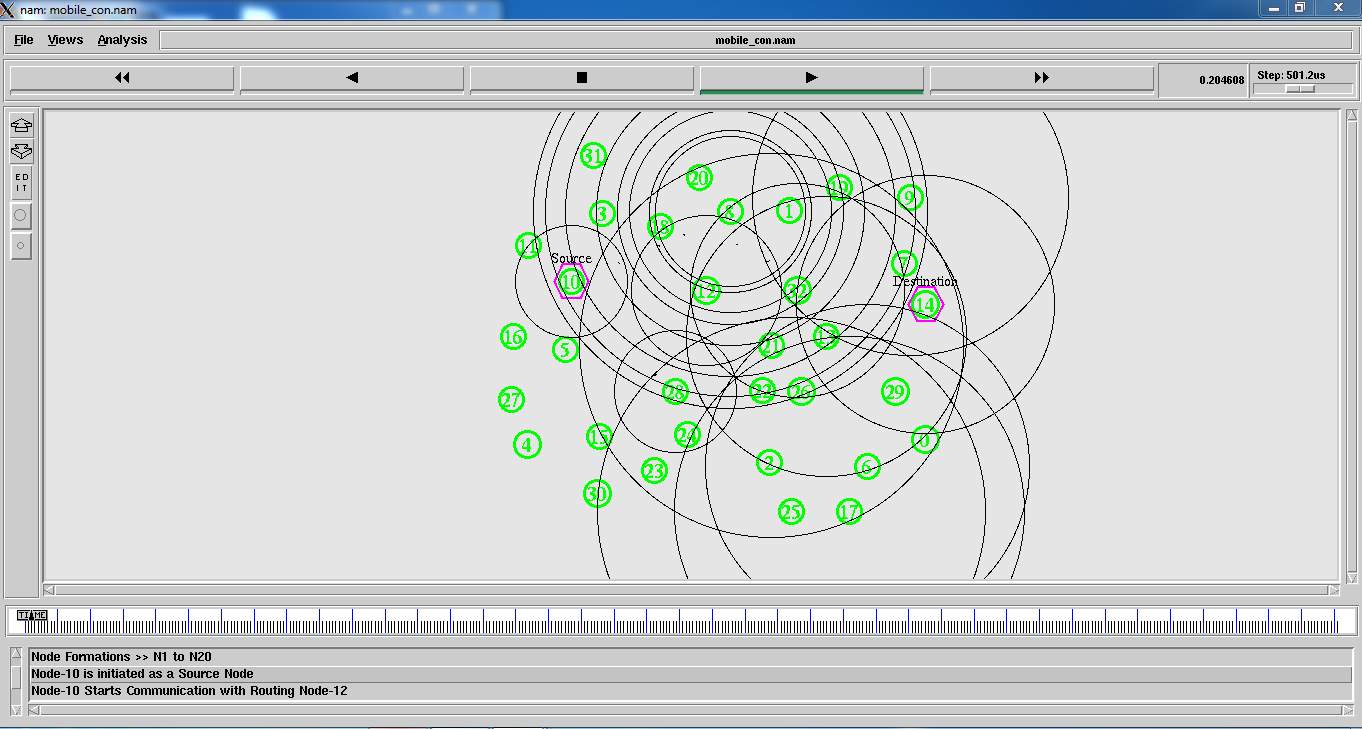
FIG 8.11.1(A) – SIMULATION 1
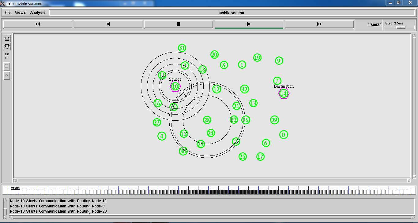
FIG 8.11.1(B) – SIMULATION 2
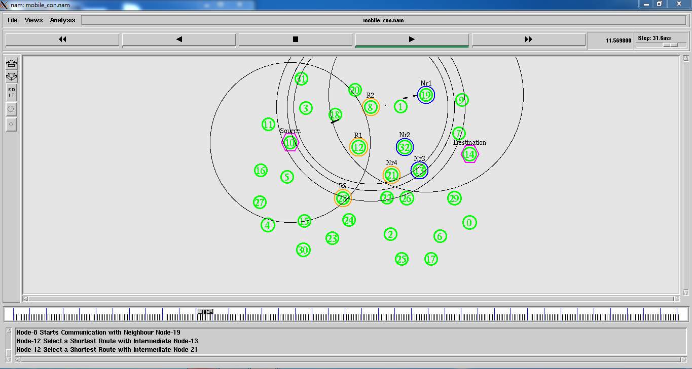
FIG 8.11.1( C) – SIMULATION 3
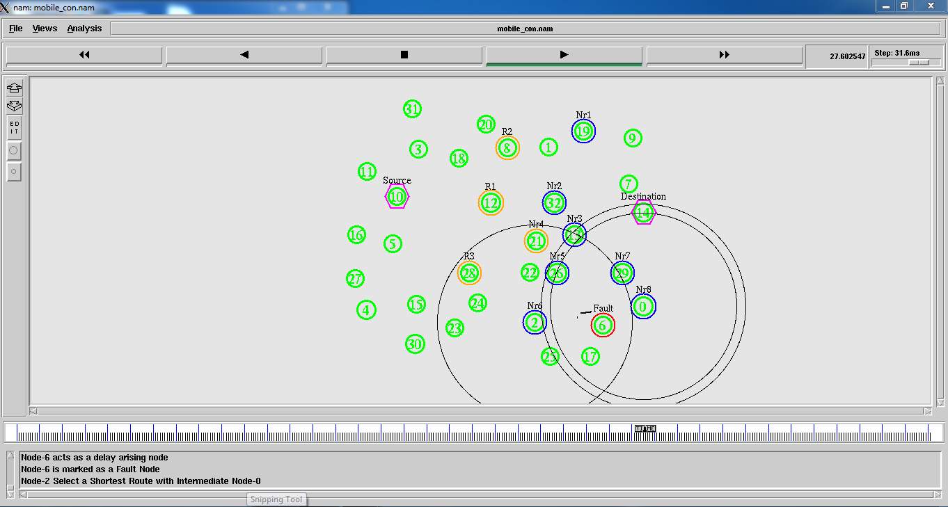
FIG 8.11.1(D)– SIMULATION 4
8.12: After the simulation ends, this is how the nodes look like.
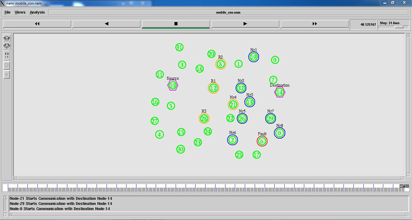
FIG 8.11.1(E)– RESULT OF SIMULATION
8.12: To access the graphs the command to be used is ns graph.tcl
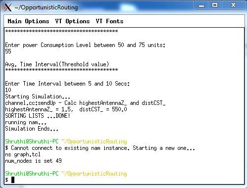
FIG 8.12.1 – TO ACCESS GRAPHS
CHAPTER 9: SYSTEM TESTING
The purpose of testing is to find errors. Testing is that the method of making an attempt to find each conceivable fault or weakness in a very work product. It provides the way to envision the practicality of elements, subassemblies, assemblies and/or a finished product it’s the method of elbow grease computer code with the intent of guaranteeing that the
Software system meets its necessities associate degreed user expectations and doesn’t fail in an unacceptable manner. There are unit numerous forms of check. every check kind addresses a selected testing demand.
TYPES OF TESTS
Unit testing
Unit take a look ating involves the look of test cases that validate that the interior program logic is functioning properly, which program inputs manufacture valid outputs. All call branches and internal code flow ought to be valid. it’s the testing of individual computer code units of the appliance .it is done once the completion of a personal unit before integration. this can be a structural testing, that depends on data of its construction and is invasive. Unit take a look ats perform basic tests at element level and test a selected business method, application, and/or system configuration. Unit tests make sure that every distinctive path of a business method performs accurately to the documented specifications and contains clearly outlined inputs and expected results.
Integration testing
Integration tests square measure designed to check integrated software system parts to see if they really run joined program. Testing is event driven and is a lot of involved with the essential outcome of screens or fields. Integration tests demonstrate that though the parts were on an individual basis satisfaction, as shown by with success unit testing, the mix of parts is correct and consistent. Integration testing is specifically geared toward exposing the issues that arise from the mix of parts.
Functional test
Functional tests give systematic demonstrations that functions tested area unit on the market as such by the business and technical necessities, system documentation, and user manuals.
Functional testing is focused on the subsequent items:
Valid Input: known categories of valid input should be accepted.
Invalid Input: known categories of invalid input should be rejected.
Functions: known functions should be exercised.
Output: known categories of application outputs should be exercised.
Systems/Procedures: interfacing systems or procedures should be invoked.
Organization and preparation of practical tests is concentrated on necessities, key functions, or special check cases. Additionally, systematic coverage touching on determine Business method flows; knowledge fields, predefined processes, and sequential processes should be thought-about for testing. Before practical testing is complete, extra tests area unit known and also the effective price of current tests is set.
System Test
System testing ensures that the whole integrated package meets necessities. It tests a configuration to make sure well-known and inevitable results. associate example of system take a look is that the configuration orientating system integration test. System testing relies on method descriptions and flows, action pre-driven method links and integration points.
White Box Testing
White Box Testing may be a testing during which during which the package tester has information of the inner workings, structure and language of the package, or a minimum of its purpose. Its purpose. It wont to check areas that can’t be reached from a recording equipment level.
Black Box Testing
Black Box Testing is testing the code with none data of the inner workings, structure or language of the module being tested. Recording equipment tests, as most different kinds of tests, should be written from a definitive supply document, like specification or necessities document, like specification or necessities document. Lets a take a look within which the code below test is treated, as a recording equipment .you cannot “see” into it. The take a look at provides inputs and responds to outputs while not considering however the code works.
9.1 TEST CASES FOR DATA SECURITY
| Test | Input | Recvd Output | Act Output | Desc |
| Encode | Data, Matrix, Sender File | Success |
Success |
Test Passed!
Data encrypted |
| Encode |
Data, Matrix, Sender File |
Failed |
Failed | Test Passed! Invalid or null data or invalid rows and cols for matrix |
|
Decode |
Encoded Data, Matrix. | Success | Success |
Test Passed! Data retrieved and displayed as text. |
| Decode | Encoded Data, Matrix. Data | Failed |
Failed |
Test Passed! Invalid password, try again |
|
Decode |
Encoded Data, Matrix. Data |
Failed |
Failed |
Test Passed! Invalid matrix, try again |
9.1.1 TEST CASES FOR OPTIMISTIC ROUTING
Filename : Main.tcl
| Test | Input | Recvd Output | Act Output | Desc |
|
Optimistic Routing |
Get the Source & Destination Node |
Find The Shortest Route |
Find The Shortest Route | Test Passed!
Find The Shortest Route |
| Optimistic Routing | Get the Source & Destination Node |
Find The Shortest Route |
Routing Failed |
Test Passed! Invalid Destination or path or Nodes Failure routes are Changed
|
9.1.2 TEST CASES FOR LINK QUALITY ESTIMATION PROTOCOL
Filename : Main.tcl
| Test | Input | Recvd Output | Act Output | Desc |
|
Link Quality |
Find the Shortest Path |
Path Node Link Strength and Speed, Time Duration to the transmission is Good |
Path Node Link Strength and Speed, Time Duration to the transmission is Good |
Test Passed! Check the Link Quality Estimation |
| Link Quality |
Find The Shortest Path |
Path Node Link Strength and Speed, Time Duration to the transmission is Good |
Node Strength, Transmission Speed and no of nodes are very large |
Test Passed! Nodes Failure Link Quality Estimation |
9.1.3 TEST CASES FOR CONGESTION MEASURE
Filename : Main.tcl
| Test | Input | Recvd Output | Act Output | Desc |
|
Congestion Measure |
Check the Congestion Measure |
Node Weight, Data Weight and Estimation Time or Good |
Node Weight, Data Weight and Estimation Time or Good |
Test Passed! Congestion Measure |
|
Congestion Measure |
Check the Congestion Measure |
Node Weight, Data Weight and Estimation Time or Good |
Node Weight, Data Weight and Estimation Time or Not Good Route are Changed |
Test Passed! Congestion Measure Nodes Link Failure!! |
9.2 GRAPHS:
The graphs that are generated from the simulation are as follows:
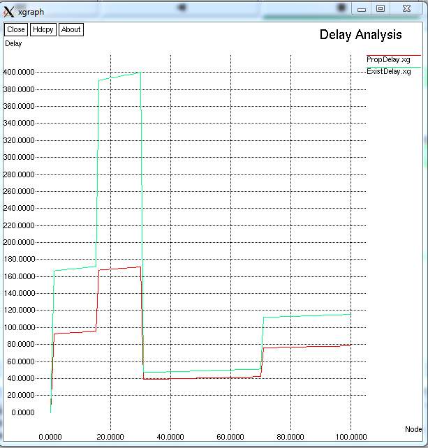
FIG 9.2.1– GRAPH FOR DELAY ANALYSIS
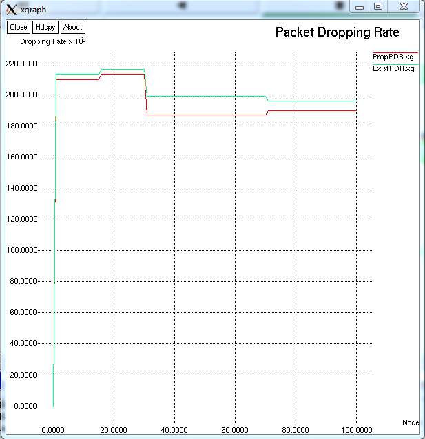
FIG 9.2.2 – GRAPH FOR PACKET DROPPING RATE
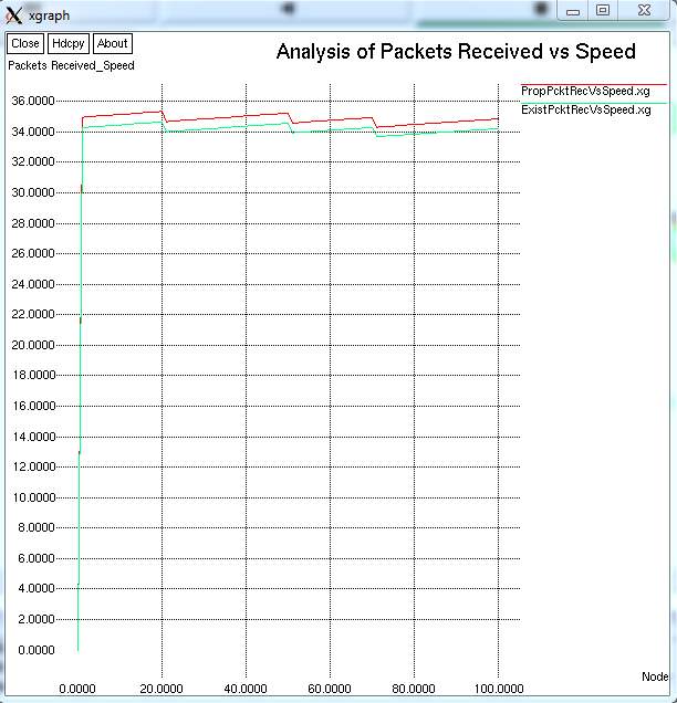
FIG 9.2.3– GRAPH FOR ANALYSIS OF PACKETS RECEIVED VS. SPEED
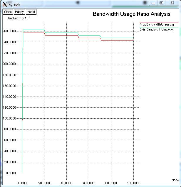
FIG 9.2.4 – GRAPH FOR BANDWIDTH USAGE RATIO ANALYSIS
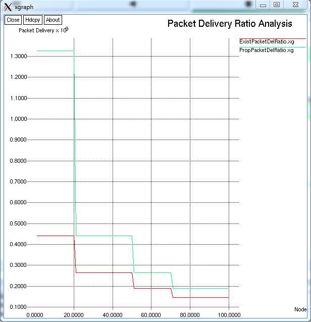
FIG 9.2.5– GRAPH FOR PACKET DELIVERY RATIO ANALYSIS
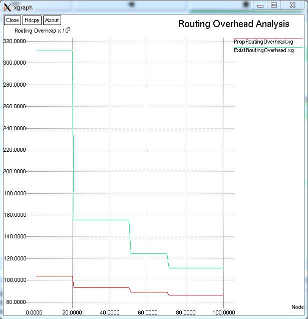
FIG 9.2.6 – GRAPH FOR ROUTING OVERHEAD ANALYSIS
CHAPTER 10: CONCLUSION AND FUTURE ENHANCEMENT
The integrated routing and MAC protocol for multi-hop wireless networks in which the best of multiple receivers forwards each packet. In this paper, combining the important aspects of shortest path routing with those of backpressure routing, we provided a distributed opportunistic routing policy with congestion diversity (D-ORCD) is proposed under which packets are routed according to a rank ordering of the nodes based on a congestion cost measure. Furthermore, we show that DORCD allows for a practical distributed and asynchronous 802.11 compatible implementation, whose performance was investigated via a detailed set of NS 2 simulations under practical and realistic networks. Simulations show that DORCD consistently outperforms existing routing algorithms in practical settings. In D-ORCD, we do not model the interference from the nodes in the network, but instead leave that issue to a classical MAC operation. However, the generalization to the networks with inter-channel interference follows directly from [7]. The price of this generalization is shown to be the centralization of the routing/scheduling globally across the network or a constant factor performance loss of the distributed variants.
In this Project, we introduced three practical modifications of ORCD referred to as P-ORCD, Infreq-ORCD, and DORCD. P-ORCD reduces the overhead cost of ORCD by restricting the number of nodes sending acknowledgments; while Infreq-ORCD and D-ORCD allow for the implementation of ORCD with low computational cost. Furthermore, we provided numerical examples to compare the performance of ORCD and its modifications with each other and also against known opportunistic routing policies. While we established the throughput optimality of ORCD, throughput optimality of modifications of ORCD remains a future area of study.
BIBILOGRAPHY
[1] P. Larsson, “Selection Diversity Forwarding in a Multihop Packet Radio Network with Fading channel and Capture,” ACM SIGMOBILE Mobile Computing and Communications Review, vol. 2, no. 4, pp. 47– 54, October 2001.
[2] M. Zorzi and R. R. Rao, “Geographic Random Forwarding (GeRaF) for Ad Hoc and Sensor Networks: Multihop Performance,” IEEE Transactions on Mobile Computing, vol. 2, no. 4, 2003.
[3] S. Biswas and R. Morris, “ExOR: Opportunistic Multi-hop Routing for Wireless Networks,” ACM SIGCOMM Computer Communication Review, vol. 35, pp. 33–44, October 2005.
[4] C. Lott and D. Teneketzis, “Stochastic routing in ad-hoc networks,” IEEE Transactions on Automatic Control, vol. 51, pp. 52–72, January 2006.
[5] S.R. Das S. Jain, “Exploiting path diversity in the link layer in wireless ad hoc networks,” World of Wireless Mobile and Multimedia Networks, 2005. WoWMoM 2005. Sixth IEEE International Symposium on a, pp. 22–30, June 2005.
[6] Parul Gupta and Tara Javidi, “ Towards Throughput and Delay Optimal Routing for Wireless Ad-Hoc Networks,” in Asilomar Conference, November 2007, pp. 249–254.
[7] M. J. Neely and R. Urgaonkar, “Optimal backpressure Routing for Wireless Networks with Multi-Receiver Diversity,” IEEE Transactions on on Information Theory, pp. 862–881, July 2009.
[8] L. Tassiulas and A. Ephremides, “Stability Properties of Constrained Queueing Systems and Scheduling Policies for Maximum Throughput in Multihop Radio Networks,” IEEE Transactions on Automatic Control, vol. 37, no. 12, pp. 1936–1949, August 1992.
[9] S. Sarkar and S. Ray, “Arbitrary Throughput Versus Complexity Tradeoffs in Wireless Networks using Graph Partitioning,” IEEE Transactions on Automatic Control, vol. 53, no. 10, pp. 2307–2323, November 2008.
[10] Y. Xi and E. M. Yeh, “Throughput Optimal Distributed Control of Stochastic Wireless Networks,” in WiOpt, April 2006.
[11] B. Smith and B. Hassibi, “Wireless Erasure Networks with Feedback,” arXiv:0804.4298v1, 2008.
[12] Y. Yi and S. Shakkottai, “Hop-by-Hop Congestion Control Over a Wireless Multi-Hop Network,” IEEE/ACM Transactions on Networking, vol. 15, no. 1, pp. 133–144, February 2007.
[13] M. Naghshvar, H. Zhuang, and T. Javidi, “A General Class of Throughput Optimal Routing Policies in Multi-hop Wireless Networks,” 2009, arXiv:0908.1273v1.
[14] E. Leonardi, M. Mellia, M. A. Marsan, and F. Neri, “Optimal Scheduling and Routing for Maximum Network Throughput,” IEEE/ACM Transactions on Networking, vol. 15, no. 6, pp. 1541–1554, December 2007.
[15] S.Shakkottai L.Ying and A. Reddy, “On Combining Shortest-Path and Back-Pressure Routing Over Multihop Wireless Networks,” IEEE/ACM Transactions on Networking, vol. 19, June 2011.
[16] L. Huang, S. Moeller, M.J. Neely, and B. Krishnamachari, “LIFOBackpressure Achieves Near Optimal Utility-Delay Tradeoff,” in Proc. of 9th Intl. Symposium on Modeling and Optimization in Mobile, Ad Hoc, and Wireless Networks (WiOpt), 2011.
[17] W. Stallings, Wireless Communications and Networks, Prentice Hall, second edition, 2004.
Cite This Work
To export a reference to this article please select a referencing stye below:
Related Services
View all


Related Content
All TagsContent relating to: "Civil Engineering"
Civil Engineering is a branch of engineering that focuses on public works and facilities such as roads, bridges, dams, harbours etc. including their design, construction, and maintenance.
Related Articles

DMCA / Removal Request
If you are the original writer of this dissertation and no longer wish to have your work published on the UKDiss.com website then please: