A Bioinformatic Approach to Elucidate Evolution of Transcription Factor Binding Sites in Drosophila melanogaster
Info: 21634 words (87 pages) Dissertation
Published: 14th Feb 2022
Tagged: Biology
Contents
Click to expand Contents
1 Introduction
1.1 Cis-Regulatory Modules definition and characterization
1.1.1 Architecture
1.1.2 Activation
1.1.3 Communication and regulation
1.2 CRM annotation and prediction
1.2.1 Bioinformatics approaches
1.2.2 Validation
1.3 Evolution of CRMs and other types of non-coding DNA
1.3.1 TFBS turn-over and TF binding features
2 Objectives
3 Methodology
3.1 Data collection
3.1.1 Raw sequences
3.1.2 Coding sequences coordinates
3.1.3 CRM and TFBSs
3.1.4 ChIP-Seq Data
3.2 Data selection
3.3 Pipeline
3.3.1 Analysis and tools
3.3.2 Sliding windows analysis
3.3.3 Concatenated sequence analysis
3.3.4 McDonald and Kreitman test
4 Results and discussion
4.1 SlidingWindows
4.2 Concatenated sequence analysis
5 Conclusion
6 Appendix
7 Bibliography
1 Introduction
1.1 Cis-Regulatory Modules definition and characterization
Gene expression has shown to be regulated by genomic structures called cis-regulatory modules (CRMs). Understanding and learning how CRMs carry out their functions and how they evolve are crucial features to finally elucidate the genotype-phenotype map of an organism.
1.1.1 Architecture
The definition of a CRM has evolved in the same way as the term gene. Initially, it was considered an enhancer, a cis-acting DNA sequence that could increase the transcription rate1. However nowadays, due to a better gene regulation understanding, the CRM concept covers the ability to regulate spatial and temporal expression pattern of genes. In the recent years, thus, the definition of a CRM has been reviewed an expand.
A CRM is a modular DNA structure of 50pb to 1.5kb that contains Transcription Factor Binding Sites (TFBSs), that regulates the transcription process. Therefore, CRM other regulator systems such as promoters, enhancers, or insulators as well as other regulator system2. For genes transcribed by the RNA polymerase II, regulatory elements include both the promoter (situated at the Transcription Start Site, TSS) and distal sequences3. However, among all the CRM types, enhancers play a major role in the initiation of gene expression, that’s why identifying these CRMs localizations has been a great challenge in many studies. Then, the CRM term is commonly used to refer to enhancers and are typically distal from the promoter.
The regulation of genes mostly implicates an interaction between TFs and CRM, and the description and differentiation of the DNA sequence to which transcription factor binds is important. A specific TFs typically recognizes small (6-12pb) DNA sequences, called TFBSs. When the associated TFs are expressed in overlapping spatial domains, the combinatorial binding and the binding cluster can result in discrete and precise patterns of transcription rate. TFs occupancy at different stages or conditions has demonstrated that TFs can often occupy diverse CRM sets and TFBSs clusters, depending on the stage and/or the conditions. Many observations have shown that it is not simply the timing of TFs expression, but rather the timing of this DNA occupancy, which controls the temporal nature of gene regulatory network4. In addition, CRMs could act across several locations at genome, and differ their relative positions to their target from a few kilobases to several hundred upstream to the promoter region or downstream. Moreover, the number of CRMs could differ between target genes, so we need to emphasize that a single gene may own one or multiple CRMs. Moreover, the TFBSs clusters will be compounded by one or multiple TFBSs too. Así pues, del tamaño total de los CRMs solo una pequeña parte es realmente ocupada por TFBSs. Las secuencias que no corresponden a los TFBSs, y que por tanto los separan dentro de los CRMs, son denominadas spacers.
In addition, in order to understand the CRM architecture deeper, two motif characteristics have been studied to understand their functionalities: motif composition and motif positioning. Motif composition is the presence within CRM of TFBSs for specific TFs. In several cases, signatures of TFs occupancy are enough to predict temporal aspect of enhancer activity. Motif positioning is the relative order, orientation and spacing of TFBSs within the CRM, and it’s often observed as strict sequence constraint. Motif positioning ensures that TFs binding facilitates the cooperative binding and protein-protein interaction, in order to ensure the proper transcriptional machinery functioning and possible co-factor recruitment4,5. If two TFs cooperatively bind to DNA through a direct protein–protein interaction, they typically need to be positioned on the same face of the DNA. This is facilitated by having a spacing of ~10 bp, 20 bp or 30 bp between the two motifs. When site 1 and site 2 are separated by spacings such as ~5 bp, 15 bp or 25 bp, the TFs will be positioned at opposite faces of the DNA helix, thereby blocking their ability to bind directly to each other.Spacing rules between motifs can also occur at larger distances, which reflects DNA wrapping around nucleosomes. TFBSs can be inferred from the motif architecture at CRMs, and the TFs occupancy has several implications in how enhancers functions.
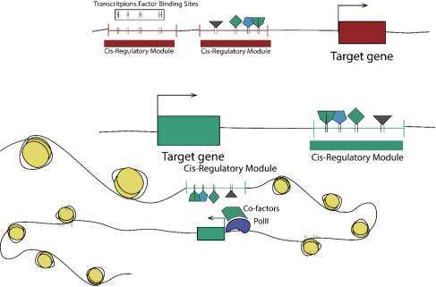
Figure 1. CRM architecture regarding target gene. CRM could act through different localization regarding a target gene. In addition, they act at chromatin at different levels and could interact with other CRM or target gene depending the case.
Box 1. Main types of CRM6,7:
Promoter: a promoter direct RNA polymerase to initiate at the Transcription Start Site. In general TFs bind to a core promoter of ~100pb around TFBS and facilitate the polymerase binding. Some core promoters contain well-known motifs, such as a TATA box, however, most promoters in mammalian genomes are GC- and CpG-rich regions that lack TATA boxes and tend to support initiation of transcription at a broad range of positions within a roughly 100 bp interval. The heterogeneity in sequence composition and genomic structure of promoters has complicated the accurate prediction of this CRM class based on single sequences. Furthermore, CpG islands are not present in D. melanogaster. However, promoters reside in chromatin with distinctive modifications, and they can be identified by mapping the start sites for transcription6.
Enhancer: they are defined by their ability to activate or repress a reporter gene transcription after transfer into a transgenic animals or transfected cells. They act independently of position and orientation, and depending on the trans-environment in a given cell, the DNA segment could switch between enhancing and silencing due to the recruitment of co-activators and co-repressors co-repressors6,7. The relative position of enhancers could vary between target genes and enhancers and genes could have multiple distinct enhancers that drive the expression depending on their TFBS motif and TFs.
Insulator: such as enhancers they act on the proper target gene, even though can be located anywhere relative to it. Their effects are limited to long-range regulatory-modules; therefore, an insulator can block the activity of enhancers and thereby reduce the gene expression. Drosophila enhancer blocking act through five different protein.
Silencers: sequence-specific elements that confer a negative (i.e., silencing or repressing) effect on the transcription of a target gene. They generally share most of the properties ascribed to enhancers. Typically, they function independently of orientation and distance from the promoter, although some position-dependent silencers have been encountered. They can be situated as part of a proximal promoter, as part of a distal enhancer, or as an independent distal regulatory module; in this regard, silencers can be located far from their target gene, in its intron, or in its 3-untranslated region. Finally, silencers may cooperate in binding to DNA, and they can act synergistically.
Locus Control Regions: The discovery of the LCR in the β-globin locus and the characterization of LCRs in other loci reinforces the concept that developmental and cell lineage–specific regulation of gene expression relies not on gene-proximal elements such as promoters, enhancers, and silencers exclusively, but also on long-range interactions of various cis regulatory elements and dynamic chromatin alterations. The LCR functions by recruiting chromatin-modifying, coactivator, and transcription complexes. 6
1.1.2 Activation
The whole CRMs set and the combinatorial TFs occupancy, can lead to diverse transcriptional outputs. These features will determine the gene expression pattern across time and cell stages.
In some cases, the whole set activation is proportional to the concentration of specific TFs (additive TFs binding), known as rheostatic model. It is the traditional way to describe the CRM effects on transcription, considering CRM would increase the transcription rate. This quantitative overview is more synergistic with genes that have basal transcription. Other cases, in contrast with those graded CRMs outputs, have a nonlinear relationship between TFs concentration and the degree of occupancy of their TFBSs (cooperative binding)2.These cases can produce switch-like effects, known as binary model. It describes the CRM as an “on/off” switch for transcription, so the CRM will increase or decrease the proportion of cells transcribing a gene, but not the initial transcription rate. This cooperative binding is associated with protein-protein interaction between TFs. Binary model have evolutionary importance, as cooperative binding can theoretically bind in the levels of individuals TFs, as long as the expression of the relevant TFs reaches a threshold4.
On the other hand, Rossi et al6 shown rheostatic and the binary model are not mutually exclusive: transcription could be rheostatic in response to a single extracellular input when either activator or repressor proteins alone were present in the cell, meanwhile, when both activator and repressor are competing for the same regulatory elements the response could turn to a binary on/off switch. Such a model considers a fundamental feature of CRMs: their function is dictated by the transcription factors bound to them, and the presence or absence of these transcription factors in the cells is dictated by the expression of other genes, the cellular environment, extracellular signaling, and so forth. In some contexts, a CRM might function to increase the amount of transcript being produced, while in others the control of even the smallest amount of transcript must be tightly regulated in an on/off way. The dual functionality of CRMs could be an important mechanism through which the same gene participates in multiple pathways and developmental contexts.
Therefore, CRMs can be classified by the activation type and the arrangement of TFs within the TFBS cluster, dividing CRM into these highly cooperative TFs binding (enhancesomes) and the more flexible and additive TFs binding functional units (billboards)7. At the enhancesome model, the recruited TFs form a highly ordered protein interface that requires a specific positioning of TFs-binding, so the assembly of the structural complex and the cooperative arrangement of TFs at TFBSs would be crucial. Disruption of a single binding site could change completely the transcription rate and consequently the phenotype. Nonetheless, most CRMs do not seem to have a such highly ordered structure, and TF binding occurs in an additive or independent manner with just some few constraints on the relative positioning on their binding sites. They have a flexible TFBSs organization, and transcriptional output is measured as the sum effect of the TFs bound. All of these are considered the billboard class and it has been commonly used to describe a lot of different active regulatory elements 2,4.
It is not possible to generalize TFBSs structures within the CRM when examining CRMs that have a given activity. This is inferred by the absence of any consistent motif positioning and by diversity in motif composition at sequence the level in CRMs with similar activities5. In that manner, specific TFs combinations can generate several outputs depending on the relative positions of the motifs regarding the whole regulatory context. In the same way, similar spatial or temporal patterns can be generated from different TFs combinations.
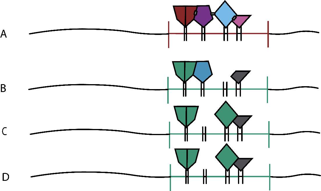
Figure 2. A: enhancesome model; the transcriptional output requires the integrated activity, correct recruitment and interaction between TFs. Motif composition and positioning need to be fix. B, C, D: billboard model; the transcriptional output requires most TFs but not all. The CRM would have more flexible composition and positioning.
1.1.3 Communication and regulation
Many regulatory interactions have been described recently, inferred from TFs occupancy patterns and comparisons between TFs binding events and expression profiles in multiple organism models8,9. Thus, some new studies suggest that even though some TFs-binding do not cause an immediate functional response, they may have a role in chromatin remodeling or nucleosome positioning, which can finally affect gene expression at a later developmental stage or have other non-transcriptional function. We need to that TFs-binding could also depend on more factors like temporal dynamics4.
In addition, CRMs act as regulatory networks. The final target gene expression will depend on the interaction among multiple regulatory elements, and the correct CRMs function depends on the interaction between multiple TFBSs. Several studies have shown that several CRM displaying similar or even identical spatial and temporal activities exist. This redundancy suggest that some target genes may include a “secondary’s” CRMs10,11.
These “secondary’s” CRMs was called “shadow enhancers” by Perry et al11. At their study, Perry et al11identified enhancers that would drive the expression of brinker and sog genes11. So after annotation and identification they determined that shadow or secondary enhancers share several features: (1) each enhancer drive the same gene expression that another previously annotated primary enhancer; (2). Bind the same TFs (there is no information about what are the TFBSs motif that they bind); (3) are located either within an intron of, or on the far side of, a neighboring gene12. So the distinction between them is purely based on the distance to the gene promoter. Both activities are commonly equivalent, and there is not any functional difference. This fact rises the hypothesis that the shadow enhancer may provide phenotypic robustness, demonstrated by the phenotypic maintenance even one regulatory module is lost13. Then, this secondary enhancer could act by shielding gene expression and can explain why deletions of well-defined enhancers produce no phenotypic effects. 8–10
Therefore several CRMs, proximal and distal to the target gene, regulate a given tartget gene, organizing and creating a regulatory network necessary for controlling gene expression. Large chromatin loops bring enhancers and target genes into proximity, leading to simple interactions. Indeed, chromatin conformation capture technologies have provided many examples of this phenomenon14,15.
The capacity to regulate target genes through proximal and distal CRM have proposed multiple models to describe the CRM communication. Three major models have been proposed: (1) DNA scanning model propose that first TFs bind to the CRM, and then the whole protein cluster within the CRM moves along the DNA sequence until it encounters the promoter. This model would be consistent with insulators elements blocking the march of the protein-complex13 [Box 1]. However, it does not explain how an enhancer located on one chromosome is able to activate transcription from an allelic promoter located in chromosome, as in transvection13,16; (2)The looping model proposes that communication between the CRM and its target genes through protein–protein interactions. TFs bound to the CRM, which in turn it would be able to contact with the transcription machinery assembled at the core promoter. This would be possible due to DNA looping2,13. Experiments using the chromatin conformation capture (3C) assay have provided direct experimental evidence of both looping interactions between distant genomic regulatory regions and intrachromosomic interactions in eukaryotic cells2; (3) the facilitated tracking model integrates elements of both of the previously described mechanisms. In this model the complex of TFs and cofactors formed at a CRM moves along the intervening sequence in small steps forming looped chromatin structures13.
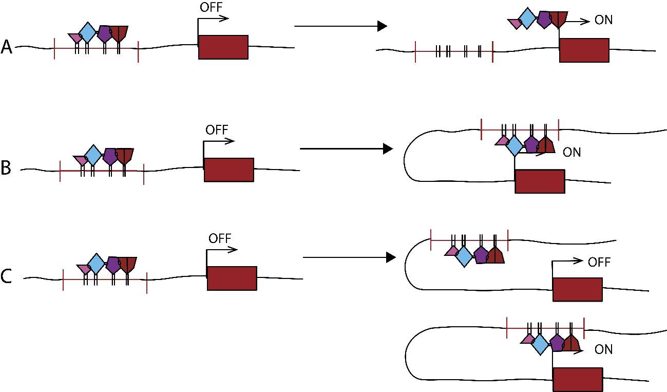
Figure 3. CRM modes of action. A: DNA scanning model; B: Looping model; C: Facilitated tracking model.
Communication and interaction among regulatory elements is an important feature in the control of gene regulation, so gaining insight into the mechanisms that govern the interactions between enhancers and their target genes will be an important step forwards. Thus, like an enhancer’s output, which can be influenced by the relative positioning of TFs binding sites, the transcriptional output may be shaped by the overall architecture of a locus, including the relative position of genes, enhancers and possible interspersed structural elements. New three-dimensional chromosomal organization approaches are elucidating this complex regulatory network. Integrating this information and discerning its functional implications are key challenges in understanding the general principles of transcriptional regulation.
1.2 CRM annotation and prediction
In spite of new technologies and progress in in silico approaches, identification, prediction and characterization of CRMs remains a great challenge. Validation and false positives are still the main problems in public databases. Regions where TFs bind contain clusters of different TFBSs which are typically used to define and identify regulatory elements, but even though any given motif present in the DNA sequence could theoretically be bound in vivo, only 1 in 500 are seen to be bound in large scale genomes 17,18. In addition the lack of information about the CRM functionalities, composition or positioning make difficult the correct interpretation and validation of the results. Quite the opposite occurs in coding sequence, where analysis of DNA, expression sequence tags and translated proteins define a context that facilitate the protein annotation.
Large scale sequencing and the availability of several bioinformatics tools have facilitated decoding the sequence that is responsible for gene regulation, as well as the intersection between in silico and in vitro analysis in model organisms. Among experimental approaches, ChIP-chip, ChIP-seq or DNAse-seq, have had a major role in TFBS mapping, as well as new 3C based studies are basic to the correct CRM localization, identification and networking interactions comprehension [CITAR]. These approaches are essential to improve the understanding and characterization of CRMs. In the same way, they are essential to elucidate the role of CRMs in the genetic regulatory networks. In silico approaches include trained models and phylogenetic footprinting (i.e. analysis of the conservation of non-coding regions across different species, considering evolutionary distance between the species17,19,20) as common features to annotate CRMs, among others.
1.2.1 Bioinformatics approaches
1.2.1.1 Motif-based
The fact that TF binding requires the presence of clusters of TFBSs motivated one of the most powerful bioinformatics approaches to annotate CRMs: the motif-based prediction. The main advantage of this method is that it can be performed by using the genomic DNA sequence, testing for models of TFBS for a specific TF. However, TFBSs are very short sequence sequences and thus putative motifs are widespread along the genomes. As a result, this motif-based prediction leads to overstate the number of true CRMs through many false positives. So, motif-based prediction of CRMs typically need other kinds of information to achieve realistic results. Given that CRMs harbor sequence features that are frequently conserved between related species, typical motif-based CRM detection methods consist in the search of two properties regarding motifs and CRM architecture: signal and sequences features, as well as the spatiotemporal relationship between them21. There exist many different software able to do that21–25. In addition, training models to discriminate different classes of CRMs can improve the inference of TFBS motifs and CRMs. The ability to discover novel TFBS motifs, especially in the process of CRM identification and classification, will remain important as long as TFBS motifs have not been comprehensively defined17.
Motif-based searches still tend to suffer from a lack of specificity and give a large number of false positives3,21,26. This somehow disappointing performance of motif-based algorithms is likely due to several factors. There are few CRMs for which the entire set of bound TFs or relevant TFBSs is known, meaning that choices of which TFs to consider may often omit relevant factors. Conversely, not all motifs found within CRMs are functionally important, including those that may have been used as input for successful motif-based CRM discovery. TFBS motifs themselves are degenerate, and the motifs for many TFs are incompletely characterized. Nevertheless, in those cases where the constituent TFBSs are well defined and well modeled, motif-based CRM discovery can be an effective approach.
1.2.1.2 Comparative genomics
Some of the most effective approaches for CRM identification use completely bypass TFBS identification, and predict CRM using only DNA sequence3,27. These kinds of approaches have been widely developed by Halfon group, and the methodology intends to determine statistical features of CRM sequences in the training set as compared to those of a background set of non-CRM sequences, and the search sequence at the genome with similar attributes3,26,27. It does not require a prior knowledge, due to the method reliance on alignment comparison, even though it requires a set of known CRMs in order to check the analysis.
In addition, despite their potential, a pure comparative genomic analysis per se needs some assumption for correct CRM prediction. Even though most functional sequences have remained more similar than non-functional DNA, showing the action of purifying selection, this is not universally true for CRMs28. In that way, evidence of strong evolutionary constraint in non-coding DNA, without other information such as TFBS motifs, has been used successfully as de novo predictor of CRMs, and there are a good number of software based on [citar+software].
As Hardison and Taylor reviewed, the combination of both sequence features and across-species alignments could result in a more comprehensive analysis of CRM prediction17. In that way, the specificity of CRM prediction was improved when TFBS motif instances were restricted to those that are conserved in other species 29,30. Although a CRM may be constrained among species, individual TFBS motif instances can tolerate sequence-level change, even to include the loss of TFBS and the gain in the flaking region 28,31–34, as we will see below. Modelling the evolution of CRMs can capture the signatures of this change without assuming sequence-level conservation. Among the many available software35, MorphMS23 model identifies regions in an existing pairwise alignment that fit an evolutionary model derived from a set of existing TFBS motifs and was found to have the best performance for recovering known D. melanogaster CRMs in a comparison of several computational approaches17,35. In addition HMM-based approaches have recently appeared36. Moreover, multiple approaches try to include sequences features again, and search for patterns in a set of known CRMs that distinguish them from non-functional DNA, facilizing the capture signatures of change rather than just constraint17. Su et al35 present a complete overview and statistical results comparing different situations and softwares. They highlight the importance of motif predictors and pre-compiled TFBS libraries and multiple genome alignment as general features to many CRMs, and compare software and combination methods. They assume that strategies for the existing methods could be classified into four families: Windows clustering, Probabilistic modelling, Phylogenetic footprinting and Discriminative modelling35.
In addition, conservation of CRM content (TFBS positioning or TFBS composition) may be more important than sequence conservation. In that way, two CRMs could be easily aligned and still their functionalities could be completely different, if TFBSs inside are incompletely conserved or spacing between them is varied.
1.2.1.3 Epigenetic
Given the limitations of methods based on sequence motifs and comparative genomics, direct measurement of diagnostic epigenetic features should lead to improved methods for CRM prediction17.
Particular epigenetic features are highly correlated with CRMs, and several approaches are doing major progress to find combinations of these features that are able to identify new CRMs. Chromatin immunoprecipitation (ChIP) is a reliable method for purifying DNA that is in close contact with a particular protein in animal cells, as long as the interactions are sufficiently stable and a highly specific anti-body is available. ChIP technologies are able to obtain in vivo profiles of TF-binding, a fact that would lead to CRM identification via TFBS-clustering3,37. This approach is appropriate when TFs and target genes are known. However, this information is currently available for only a minority of developmental systems. With the introduction of sequence consensus methods, in which the immunoprecipitated DNA is analyzed on massively parallel short-read sequences, the DNA that is in close contact with the protein of interest can be determined with remarkable sensitivity and resolution (200–300 bp) across an animal genome. An intriguing discovery has been the presence of ‘HOT’ (highly occupied target) regions, in which unexpectedly high numbers of different TFs are observed to bind3,37.
A related CRM discovery strategy is to use ChIP-seq to identify the in vivo binding sites of transcriptional coactivators, such as the acetyltransferase p300/CBP 3,17. This approach does not requires to knowledge of the TFs, and thus it could facilitate the de novo TFBS annotation. Because not all TFBSs are bound in specific stages or tissues, and because of the use of a generic coactivator, we need to keep in mind that this technique does not allow the discovery of all active CRMs. Another variant of ChIP-based methods is to target the various post-translational modifications (PTMs) seen on the tails of histones in the nucleosomes flanking CRMs3. The number of studies using this method for CRM identification has risen dramatically. Several studies have interpreted the combinations of histone PTMs further, and they identify active enhancers based on the presence or absence of modifications.
Lastly, chromatin accessibility is another important fact of gene regulation. Active CRMs are regions of nucleosome-depleted ‘open’ chromatin and can be identified on a genome-wide scale through several of methods38. DNase-seq, which is sensitive enough to resolve individual TFBSs, makes use of the enhanced susceptibility of open chromatin to enzymatic cleavage by DNase I in a genome-wide, next-generation sequencing-based extension of traditional DNase I footprinting and hypersensitivity assays39.
As collections of TFs and their cognate TFBS motifs are more completely defined, a promising future direction is to build quantitative models that predict expression levels under diverse conditions for both naturally occurring and synthetic CRMs.
1.2.2 Validation
High throughput assays as prediction models have raised the number of putative CRMs annotated in the genomes. To validate CRM annotations and to create specialized databases are major challenges nowadays in this topic. In this way model organism and cell lines in culture are being used to measure CRM activity and networking, and lastly CRM validation.
Transferring a DNA segment in a reporter gene into cultured cells or whole organism is still one of the most common methods to test the regulation ability in gain-of-function assays. Transgenic assays and Genetically Modified Organisms (GMOs) can be used for comparison of CRM functionality across species, which can elucidate evolutionary information. Invertebrates have been used typically to generate maps of networking regulation in development and to define the CRM logic and interaction2,38,40.
As Jeziorska et al reviewed, another powerful approach to understand CRM networking, basic logic and dynamics could be live cell imagining and live organism imagining. CRMs can be used to drive expression of fluorescent/luciferase reporters in cells in culture and their activity quantified in real time with single-cell resolution. In this way, measurement noise inherent to other populations cells transcripts is eliminated and gene expression is visualized at the level in which transcriptional decisions are made. Moreover, confocal and multi-photon microscopy have recently been adapted to time-lapse studies of entire model organisms. Few selected examples measuring the dynamics of oscillatory gene expression are referred to at the paper, and ratify the live cell imaging approach to validate CRM function2,41.
1.3 Evolution of CRMs and other types of non-coding DNA
Understand the functional significance and evolutionary forces governing CRMs and other non-coding region is nowadays a great challenge in genomics. Considering the information available and the role of CRM in gene expression, in addition to the fact that the high degree of protein similarity between phenotypically diverged species have led to propose that regulatory evolution could be more important than protein evolution, and a fraction of non-coding DNA would be crucial on the process (especially mutations affecting TFBS and CRM)42. For several theoretical reasons, TFBS and other cis-regulatory sequences may be particularly important in evolutionary adaptation. CRM determine how a protein-coding gene is expressed in any tissue. Because they encode such critical spatio-temporal and quantitative information, they are expected to be under strong purifying selection and mutate at a slower rate than flanking neutrally evolving regions. Even though enhancers tend to be evolutionarily conserved, in general they evolve faster than coding regions, suggesting that changes in regulatory DNA play an important role in evolution43. Furthermore, cis-regulatory mutations are often co-dominant, which may allow natural selection to act on them more efficiently than on protein-coding mutation. Therefore, several authors have shown that phenotypic changes may be driven by cis-regulatory mutations rather than protein-coding mutations44.
Intergenic sequence studies show that regulatory sequences are involved in chromatin organization and transcription and occupy a much larger fraction of the genome than protein coding sequences. Through the interpretation of several results and the annotated evidence for functional constraints on regulatory sequences, it seems plausible that CRM co-evolve with their core promoter in both sequence-specific and localization to achieve the best possible functional performance38. Through the molecular evolution rules described by Kimura45, conservation and evolution in non-coding sequences should imply functional constraint on these sequences, and then slower rates for molecular evolution43. There are many examples of diverged regulatory sequence, that preserve functionalities and expression patterns. Drosophila even-skipped stripe 2 enhancer (eve s2e) was one of the first non-coding DNA evolutionary example developed. In that case comparison showed that most functional binding sites were conserved at sequence level among Drosophila species28. So, they presented here a case were no single binding site were completely conserved and moreover, some functional binding sites could be gained or lost. So, signature of selective constraint is manifested as reduced levels of polymorphism and divergence, and excess of rare variants, measurable by reduced interspecies substitutions rates or the suppression of the frequency of derived alleles within a population. Trying to understand this conserved non-coding sequence constraint, another significant approach was performed by Andolfatto42.At the study, he performed a modified McDonald and Kreitman Test to check divergence within, and between species to distinguish between variation of mutation rate under neutrality and signatures of negative or positive selection. It was one of the first study at population-level variability showing that proportion of nucleotide divergence in non-coding sequences had been driven to fixation by positive selection. Then, as reviewed Ludwig43 multiple evolutionary hypotheses have been proposed to explain the observation concerning evolutionary changes in CRM.
Even though purifying selection would keep transcriptional enhancers evolving slower in relation to other non-functional DNA, CRM would change by the accumulation of mutations46. Moreover, new enhancers can appear by chance when random mutations create clusters of TFBS or lost when large deletions eliminate these sequences. Such processes can be driven by natural selection as well as purely neutral mechanisms. Turnover of TFBS in enhancers as well completely apparition or loss of CRM cause the regulatory element repertoire to change over evolutionary time46. In any case, patterns of recent evolution are really needed to learn how these non-coding DNA are conserved, and finally understand how they evolve. Then a few modified versions of test for natural selection could be applied, using nucleotide variation to study it within the same specie or some closely related one43,47,48.
1.3.1 TFBS turn-over and TF binding features
At this point, we need to keep in mind that individual and grouped TFBS have shown several times to be required for the correct function of the CRM, despite in several studies authors have checked that TFBS are able to evolve quickly and frequently33,34. In that way, inside a specific CRM, TFBS loss and gain is a common fact, and could affect the CRM functionality. This TFBS gain and loss is known as turn-over31,33. In cases where CRM function have been preserved despite sequence and structural divergence, these observations raise question about the evolutionary forces driving non-coding sequences31,42,49. One possibility for reconciling conservation of CRM function with TFBS turn-over is to assume each loss of a TFBS is balanced by analogous binding site inside the CRM by compensatory mutations (idea based on the model proposed by Kimura45, where he considers a pair of tightly linked mutant genes that are individually deleterious but in combination restore wildtype function). Trying to apply this resolution to TFBS, the gain of TFBS carrying a mutation that decrease the quality of an existing TFBS can offset the mutants’ fitness cost, creating a selectively neutral double-mutant allele. This kind of turn-over would be achieved purely by genetic drift, maintaining the CRM functionality31.
So, starting from the prevalent thought, which establishes that the elevate occurrence is due to compensatory mutations, is opposite to the fact that the turn-over could be subject to diverse evolutionary forces. He et al31 propose that it should be described a realistic model which reconciles the finding of selection driving TFBS turn-over with constrained CRM functionality over long evolutionary time. In that manner, they described new patterns of polymorphism and divergent inconsistent with neutral or nearly neutral theory, and several evidences that show the contribution of positive selection in the gain of TFBS and purifying selection in the loss of TFBS. In addition, as it’s described in Arbiza et al44, we need to consider that the analysis of conserved noncoding sequences regions could tend to dilute the signature of natural selection and makes it more difficult to connect DNA mutations with fitness-influencing phenotypes, because polymorphisms are sparse and provide weak information at individual binding sites, which can produce significant statistical biases, or they have relied on divergence patterns over longer evolutionary time scales which can be influenced by binding site turnover, alignment errors or miss identifications of orthologs.
On the other hand, Sabarinathan et al50have recently shown that mutation rate is significantly higher in TFBS and nucleosomes in comparison with flanking regions. They present robust results showing that the TF and histones junction hinder the correct performance of the Nucleotide Excision Repair system (NER), fact that causes the rise of the nucleotide mutation.
2 Objectives
We decided to start from ideas and results exposed at articles previously published, as well described at the introduction. Thus, regarding this we have two new ways to understand the CRM and TFBSs behavior (kreitman;bigas).
In that way, we try to perform a more complete analysis using updated databases, and trying to select the vast majority TFBSs and CRM possible at them. In that manner, the total number of interesting position increase significantly. In addition, our study will not focus at the merely gain and loss of TBFS through their affinity-increasing or affinity-decreasing mutation observed, but rather we will try to understand and check how are acting the diverse evolutionary forces at these constrained positions, as well as at their flaking regions. We would expect both TFBSs maintaining and gain or loss of cognate TFBSs would have a completely different evolutionary behavior, and then it could be reflected at the estimators we are going to use.
In addition we want to highlight the incorporation at this study the differentiation between those sites putative active (TFBSs bound by a determinate TFs) and those not putative active (TFBSs unbound. Considering that bound TFBSs and nucleosomes are subjected to a lower nucleotide repair rate, due to the absence of NER, we need to assume that those TFBSs and CRM directly related with germinal lines should transfer higher mutated alleles at these positions. Thus we will try to use ChIP-seq information at germinal line level, and then differentiate between bound and unbound TFBSs. Each TFBSs class must to differ at divergence and polymorphic levels, and moreover, we expect that evolutionary forces driving the CRM and TFBSs sequence and functionality constraint would be significantly different. It would be reflected at polymorphism and divergence patterns, as well as natural selection tests.
To sum up: 1. we will try to check to what extent the TFBSs turn-over are subject to positive or purifying selection regarding the TFBSs positions and their flaking region; 2 how would TFs bound affect in polymorphism and mutation rate? These features will allow us to understand the TFBSs functionality and behavior over the evolutionary time, expecting that the TFs bound would cause higher polymorphism and divergent patterns highlighted by the lack of NER system, and then showing differences at major forces driving TFBSs evolution at bound and unbound TFBSs.
3 Methodology
To perform our analysis, we need to access different databases; some of them used by previous authors. It will enable the implementation of new remarkable information for the purpose of obtaining new and more complete results.
3.1 Data collection
3.1.1 Raw sequences
In order to extract the relevant positions for our study, we accessed the raw sequences in fasta format included in Drosophila Genetic Reference Panel51. Due to the data availability at the Bioinformatics and Genomic Diversity group, we obtained the dataset through the server which store all the data included in the genomic browser PopFly52. This dataset has an amount of 205 sequences that will be use as ingroup in the following analysis. The files were modified to include a reference sequence (FlyBase D. melanogaster chromosomes assembly version 5.57), as well as an outgroup sequence. The used output sequence were the chromosome sequences of Drosophila simulans related to the assembly version 2 (Hu et al53). We chose D. simulans as outgroup mainly due to their phylogenetic relationship with D. melanogaster and their assembly quality. The outgroup sequences were previously aligned with the assembly version 5 of D. melanogaster, which allows their use for the following analysis.
3.1.2 Coding sequences coordinates
We could obtain the D. melanogaster assembly 5.57 annotation file through FlyBase database. It will be used to extract the coordinates of the Coding DNA Sequences (CDS).
3.1.3 CRM and TFBSs
In order to obtain all the data referring to CRM and TFBSs, we decided to access to REDfly database, from where we downloaded the whole annotated files of CRM and TFBSs in gff3 format. REDfly is a curated database of D. melanogaster CRM and TFBSs. REDfly database intends to include all the verified experimental results about regulatory elements over the DNA and the associated genes. Regarding the CRM annotation, REDfly focuses on those sequences with a minimal length, which have shown to be sufficiently large to regulate the genetic expression through reporter genes in transgenic animals. Due to the presence of nested sequences with identical activity, those smaller where selected and defined as CRM. Regarding the TFBSs annotation, the authors have expanded their previous annotations using electrophoretic mobility shift assays (EMSAs, gel shift), in addition to the sites annotated by DNase I footprinting. In spite of the data obtained by EMSA, the assay could not be as accurate as DNase I footprinting. However, in most cases, the authors have provided a presumed binding sequence within the probe, and they have used this to represent the binding site54.
For our approach one of most important feature, and partially, the reason whereby we decided to use REDfly is the Regulatory element-target gene positional54. The database reports the position of each regulatory element in relation to each of the transcripts of its associated gene. The coordinates of each element are evaluated against the most current genome annotation to determine whether the element lies 5’ to, 3’ within an intron of, or within (or overlaps) the transcribed region of each associated transcript.
Finally, we want to highlight that REDfly has 16180 CRMs associated with 630 genes, and 2070 TFBSs bound by 158 transcription factors associated with 214 target genes. Due to these numbers and the curation, REDfly is a powerful database for our analysis.
3.1.4 ChIP-Seq Data
In order to expand the approach, we add two new variables to check the potential differences between them. Thus, we add to results the distinction between those TFBSs which could potentially have a TFs bound at the TFBSs and those that have not any TFBSs bound. To do that, we decided to use the data expose in modENCODE: Chromatin Binding Site Mapping of Transcription Factors in D. melanogaster by ChIP-seq (Pi: Kevin White Labs: Kevin White). The intersection of coordinates from REDfly and the coordinates from ChIP-seq data will be used to elucidate the TFBSs bound and unbound. Those TFBSs present in both data will be consider as bound, and those TFBSs only present at REDfly will be consider as unbound.
3.2 Data selection
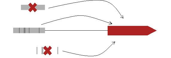
In order to obtain the expected results, first we need to clean all the raw data obtained from REDfly. When we checked the raw data for the first time, we saw quickly that we had three different cases regarding a target gene:
- First it could be possible to find a target gene with annotated CRM but no TFBSs.
- Second it could be possible to find a target gene with annotated TFBSs but no CRM
- And finally, those cases where the target gene had annotated CRM and TFBSs
TFBS
Figure 4. Possible cases at REDfly annotation file regarding a target gene.
In order to do a complete and more complex analysis we will see the following cases. In this way, from the initial set of 16180 CRM associated with 630 genes and 2070 TFBSs associated with 214 genes, the analysis will just include those target genes with CRM and TFBSs (step 1). Moreover, only the CRM with TFBSs inside will be included in the analysis. (step 2). And to expand the approach, we add the differentiation between positive and negative TFBSs (step 3)

3.3 Pipeline
3.3.1 Analysis and tools
The analysis and the tools used have followed a simple structure which, from my point of view, is intended to provide a simpler way for the total comprehension of the pipeline execution. Thus, this pipeline is based on the creation and modification of documents and results, in such a way that the programming languages and tools used follow the next logic and structure:
- Bash will be used as the language for the main script, the one we access to execute the whole pipeline, although it has different parts.
- R language will be used for statistical operations, data visualization and coordinates acquisition (coordinates will always be extracted through the Bioconductor library GenomicRanges).
- Python language (version 2.7) will be used for all the tasks which need more complex informatic treatment.
- Finally, we will use Variscan 2.0.3 as main tool to calculate polymorphic and divergent estimators.
Therefore all the tools used in the pipeline were: Variscan 2.0.3, Bioconductor library GenomicRanges, Samtools and bash, R and Python custom scripts.
Table 2. Tools and languages
| Part | Language, tool |
| Main script
Files and directories |
Bash |
| Sequences extraction | GenomicRanges and bash |
| Sequences recodification and format changes | Python |
| Data analysis | Variscan 2.03 and R |
| Data visualization | R |
We decided use Variscan rather than other possible software such as DnaSP or Popgenome, which also can calculate different polymorphic and divergent variables, due to his versatility and flexibility. First of all, for Variscan a list of different scripts is programmed, although you can use a Graphical User Interface, and thanks to this we can automate and custom in a simply way all the analysis. In addition, Variscan has different outputs modes, configurable through the track that the author denominated Config File55. In our approach, we decided to use the output modes: run mode 12 and run mode 21 (appendix, Variscan config parameters*). Such outputs modes present the different variables we want to measure: S (Segregating sites), Pi (nucleotide diversity), K (Divergence corrected by Jukes-Cantor) and Tajima D.
Once this has been said, the main reason to use Variscan and not other software relies on the possible configuration of the variables FixNum and NumNuc in the Config. Firstly, in order to use them we need to declare the variable CompleteDeletion as 0. This option allows us to include all the sites with gaps and undetermined nucleotides in the analysis. FixNum = 0 will allow to analyze a minimum number of sequences, this minimum number will be defined at NumNuc. In this way, regarding our ingroup dataset we decided to use a NumNuc = 150. So, if a given position has less than 150 nucleotides to include in the analysis, it will be discarded. On the other hand, if a given position has more than 150 nucleotides to analyze, Variscan will choose 150 nucleotides randomly, but it will always maintain reference and outgroup sequence. A 150 NumNuc value was chosen after checking manually that the vast majority of sites were not excluded by Variscan. These features allow us to maximize the number of analyzed sites.
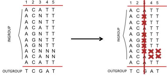
Figure 6. Variscan sitios descartados y posciones aceptadas.
We need to emphasize that Variscan cannot use fasta files; it only receives MAF, MGA, PHYLIP, XMFA OR HapMap genotype format as input files. So, another critical step before performing the analysis is transforming properly our fasta DGRP files. In our case we use a Python custom scriptin order to create the new files.
3.3.2 Sliding windows analysis
Once we have the correct coordinates and files, the first step is the analysis of the CRMs. Variscan includes its own scripts in order to select regions inside full chromosome files. So, we can create a specific block data file (bdf) with gff2dbf.pl Variscan script, and add each CRM by target gene. With this step, we could improve the Variscan performance due to it will search the regions at the bdf file and just select the coordinates inside the full chromosome file, without the necessity to extract each region in different files. In addition, the gff2dbf.pl script was also modified in order to increase the analysis performance.
Our CRM analysis estimates Pi, K and Tajima D as well as S (segregating sites) in each CRM. The whole analysis was performed with two different Sliding Windows configurations at Variscan; at first, we decided to use a WindowsSize=100 and Jump=1, for the second one we decided to use a WindowsSize=10 and Jump=1. With these two different approaches, we can visualize correctly all the CRM regardless their sizes. All the results will be included in an R custom script by target gene. Furthermore, we will be able to visualize all the TFBSs positions inside the CRM. Altogether, it allows us to check the polymorphism and divergence patterns inside each CRM.
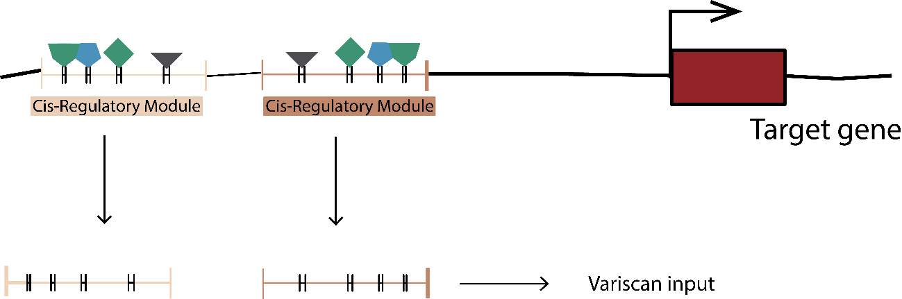
Figure 7. Example of CRM analysis.
3.3.3 Concatenated sequence analysis
Due to the TFBSs size, we need to use another approach in order to estimate the different variables correctly. An extremely small size could cause future problems in other approaches or calculations, mainly due to the lack of segregating and/or divergent sites. To solve this, we decide to analyze the TFBSs by target gene, concatenating their sequence in a new fasta file. It could be correctly performed using an R custom script again (GenomicRanges, in order to extract the coordinates) and bash custom scripts and tools (Samtools 1.5, in order to extract and concatenate the proper TFBSs in a new fasta file). Once more, the fasta file needed to be transformed to a new Phylip file.
In addition, we not only decided to analyze the TFBSs. We really thought the patterns behavior of the flanking TFBSs sequences that we denoted previously as spacers sequences, could be interesting and decisive to understand the turn-over and natural selection of TFBSs. Same as before, we decided to concatenate the spacer sequences and perform the same analysis we did with the TFBSs sequence.
In this case, even though the variables calculated by Variscan were the same, we configured the Config File without WindowsSize or Jump, because of the TFBSs concatenated size.
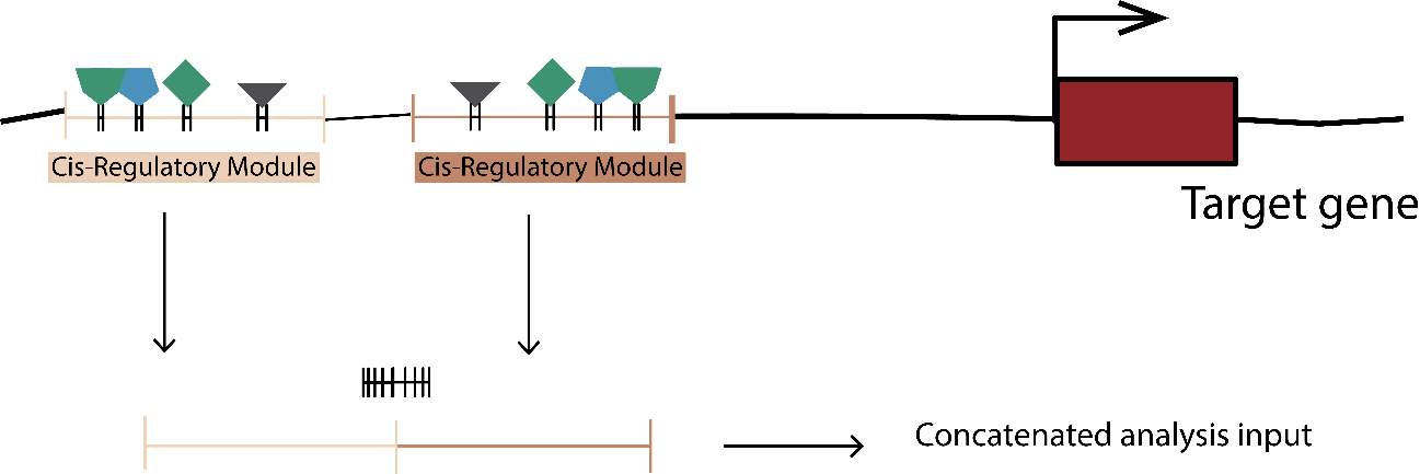
Figure 8. Concatenated tfbs and spacers
3.3.4 McDonald and Kreitman test
In order to check the amount of adaptive evolution within a species and the proportion of substitution that resulted from positive selection, we decided to perform the McDonald and Kreitman Test (MKT). MKT allows the comparison of pattern of polymorphism and divergence to elucidate selection at the DNA level. The test is based in the comparison of the amount of variation within a population to the divergence between the species at two different kinds of sites: one putative neutral and another one putative selected. Initially, Synonymous positions in a coding region were considered as the putative neutral and non-synonymous sites were considered the putative selected sites, although the test can potentially be extended to any two types of sites, considering that one of them is assumed to evolve neutrally, and that both types of sites are linked in the genome. In addition, the test can be used to analyze multiple loci simultaneously providing the appropriate multi-locus statistical tests56. Thus, our analysis will consider three situations, which always maintain the 4-fold sites as the putative neutral:
- 0-fold sites: the test will be performed in a classical way, using the coding sequence of the target gene. In this case 0-fold will be used as putative selected sites.
- TFBSs: concatenated TFBSs positions will be used as putative selected sites.
- Iii. Spacers: concatenated Spacers positions will be used as putative selected sites.
In this way, we try to check the amount and direction of adaptation at TFBSs sites. Tests 0-fold versus 4-fold were used as reference, in order to check previous results. Bioinformatically, the MKT was carried out considering different points. First, we needed to manage all the information presented at the 5.57 gff3 D. melanogaster annotation file, in order to extract and create a CDS annotation file. This file would be used to extract the largest transcript of each gene, in this way we tried to use the maximum coding positions. Again, these tasks related to manipulation and creation file were performed with bash.
The recoding of the sequence to 0-fold and 4-fold was performed with Python. In this case, the script read the sequence by codons and transform the codons to 0 and 4-fold using a Python dictionary based on the amino acid code. In this way, we created the 0-fold file avoiding the rest of the positions, changing it to undetermined nucleotide. We created the 4-fold sites in a similar way.
The necessary information to develop the MKT was obtained using Variscan (in order to get the segregating sites (S), Pi and K) and R custom script (in order to get the Minor Frequency Allele, divergent sites, and execute the test). In order to check the Variscan results, the R script integrates another segregating sites calculation. In the majority of cases the results were the same and no bias were introduced by the randomly nucleotide selection in Variscan.
Standard and integrative MKT were performed in this way.
4 Results and discussion
Our pipeline includes two main approaches in order to test the proposed objectives. Prior to start the analysis, we needed to clean up the raw data obtained from REDfly. As presented in methodology section (3.2 data selection, figure 4 and table 1) we checked different cases at the raw data, and we selected only those target genes with CRMs associated to them and those CRMs containing TFBS. At this point the first problem appeared. As it is shown in Table 1, from the 16280 annotated CRM, finally we only used 1183. These 1183 CRM are those which fulfil the proposed conditions. Therefore, we are losing 15627 annotated and validated CRMs, as well as 477 target genes.
So in order to check this loss of information, we intersected the files again, but we decided to use bash tools (BEDtools 2.18[quinlan], Bedops 2.4.26[neph] and custom AWK script) instead of using the GenomicRanges package. The results intersecting the files on our terms were the same using all different approaches. In addition, and more importantly, the pipeline performance using BEDtools and Bedops was significantly higher, the usage difficulty was quite lower. In summary, the integration as bash tools of these software provides better application on the pipeline. So, to understand what was happening, we manually checked the annotation file. The information loss is mainly due to the fact that the vast majority of CRMs are annotated to a target gene, but this target gene in several cases was an “Unspecified Target Gene”. So, even though we were cleaning up correctly the annotations files, this loss of information was unavoidable as we need the target gene to perform correctly the concatenated sequence analysis and the standard and generalized MKT(MKT) [mackay].
First, we thought we could pass this problem by associating the different CRMs with their neighbouring genes, under the assumption that by definition they are acting in cis. But, firstly we do not know if all CRMs with Unspecified Target Gene act as an enhancer, so we cannot determine if the target gene would be the one up or downstream form the CRMs coordinates. Even though the assumption it is not completely correct, it could be a good way to retrieve more information to extend our approaches. But, even assuming almost of all them were enhancers, the number of TFBS annotated on raw data are significantly lower than the CRMs, and hence we were just losing 214 TFBS from the initial set of 2070. In other words, although we can retrieve under some assumption a high number of CRM, the number of TFBS annotated would be inconsistent with the number of CRM, and finally we would discard again a high number of CRM as most of them would not fulfil our first condition (target gene with annotated CRMs and TFBS within these CRMs). In this way we tried to find a solution to retrieve the most information possible, but most important and the main reason whereby we did not do some of the explained options, it because of we would lose the robustness provided by REDfly.
4.1 SlidingWindows
First approach tries to analyse whole CRMs set by target gene in a Sliding Windows analysis. In this way, we perform an analysis with Variscan under the conditions explained at methodology. The calculation of Pi, K and Tajima D were satisfactory in almost the cases. Due to the average size of CRMs and the chosen parameters, we find some windows where there were not Segregating Sites. In this way, we obtained several examples were Pi and K had a value of zero, and moreover due to the nature of Tajima D calculations, cases where Variscan could not perform correctly the calculations. In addition, several differences exist between CRM size, so determine a correct Sliding Windows size to normalize calculation and imaging were a problem too. Therefore, we tried to visualize the Sliding Windows results displaying the TFBS positions at CRMs (Anexo images sliding). With this approach, we expected to find consistent pattern at the TFBS position. Through the visualization of the vast CRM majority, we could not elucidate any kind of pattern. It would have been interesting and expectable to observe same patterns through CRMs, or at least same pattern between CRMs regarding a specific target gene. Moreover, to infer pattern at TFBS within the CRM would have be the most interesting feature. So, due to the CRMs size, Sliding Windows calculations and the lack of significant information or estimators pattern among CRM and TFBS, we considered impossible to infer or correlate any information at the Sliding Window approach.
In our opinion, next Sliding Windows approaches will need handle the CRM by target gene concatenating and using them as input. In this way, we could normalize the windows size and visualize CRM correctly. In addition, we could increase the windows size and then, provide a solution to those windows where we cannot estimate Tajima D or other estimator due to the absence of segregating sites. Another option may be concatenate the CRM by chromosome or by recombination values on these areas, with the same purpose explained above.
4.2 Concatenated sequence analysis
As we explained, through the concatenated analysis we try to analyse TFBS and spacers positions. To perform an analysis using TFBS independently wouldn’t have been significant at most cases. TFBS are short region of DNA (6-12bp) which TF are recruited and are commonly constrained at sequence level. So, it would be expected the absence or a low number of segregating sites. It would lead into introduce biases in our results. Due to these feature, we decided to analyse them concatenating. This concatenation allows to increase the number of positions to analyse and consequently the number of segregating sites and/or divergent sites. Spacers were concatenated too, in order to be consistent with the analysis, even though almost the spacers are sufficiently large to perform the test as independent sequences. Those spacers not sufficiently large to use independently are consistent with enhancesome model [ref], where the spacing between TFBS need to be sufficiently short to allow the interactions between TF once they are the proper positions.
In this way our concatenated sequence analysis comprise three main parts: first the differentiation between bound and unbound TFBS to perform the correct analyses; second detect natural selection and evolutionary forces acting on these areas (performing standard and generalized McDonald and Kreitman Test [MKT])[mackay]; and finally the estimation of nucleotide variation (including pattern and correlation of nucleotide diversity [pi] and divergence corrected by Jukes-Cantor [K]).
So, as we explained at our objectives, we consider a key element the differentiation between bound and unbound TFBS. This distinction could be essential to elucidate how take place the turn-over in addition to understand how affect a higher mutation rate at the CRM evolution. So, those TFBS with a TF bound directly related with germinal line would reflect over evolutionary time a higher mutation rate, and then different evolutionary forces (to maintain or gain and loss TFBS). Here it is presented the main problem of our approach. In order to achieve this TFBS class differentiation we turned to modENCODE, with the purpose to obtain a chromatin binding site map. We expected to find that information referent to ChIP-seq experiments in germinal lines (or even DNase-seq which could be a good substitute to our approach). Conversely that occur with functional genetic human annotations[encode], at Drosophila, information related to ChiP-seq and binding assays are not performed by tissues or specific cell lines. Instead, the approaches are based on whole organism specific development stages. So, the at the moment only two complete annotated files referred to Binding Site Mapping are submitted at modENCODE: one performed by ChIP-seq and the other one performed ChIP-chip[ref]. modENCODE project try to generate a comprehensive annotation of the functional elements in the C. elegans and D. melanogaster genomes[modencode]. In this way we cannot perform the characterization of bound and unbound TFBS directly related to germinal line or specific tissue, which would be related with a higher mutation rate, a specific sequence constraint and different evolutionary forces that would have to be tested. Due to the lack of the proper information we decided then execute a less exhaustive approach using, as we above-mentioned, the complete ChIP-seq data submitted at modENCODE by Kevin White Labs[ref]. Kevin White Lab aims to map the association of all the transcription factors on the genome of Drosophila melanogaster. This file contains 48447 unique protein binding sites entries from a total of 72 ChIP-seq experiments. This information it’s that was used to differentiate between bound TFBS and unbound TFBS. Therefore, such as the correct data is not available, our approach cannot really test currently neither the major role of TFBS bound on CRM evolutionary features nor the higher mutation rate at these positions. Thus, although the following results are not exactly the expected, and they just test partially our objectives, we consider necessary to test our approach and the pipeline, in order to check his potential to execute next related analyses with the correct data.
As we present at Table 1, the approach was performed for a total number of 156 target genes. In order to normalize and standardize the results, we decided to include another filter. So finally, we checked just the results for those target genes where CRM contained Bound and Unbound TFBS. Then the final analysis was performed for a total of 36 target genes (anexo II), including 13002 TFBS positions of the initial 22616 positions (Table1).
In this way, we followed the steps explained at the methodology in order to perform the standard and generalized MKT. As widely explained at Mackay et al51, performing standard MKT, null hypothesis of neutrality is rejected when Di/D0 > Pi/P0, or Pi/P0 > Di/D0 (D= divergent sites; P=polymorphic sites; i=putative selected; 0=putative neutral)51. At the first case, there would be an excess of divergence relative to polymorphism regarding the putative selected sites. Then, the fraction of adaptive fixations (α) is estimated as 1 – (Pi/P0)(Di/D0). On the other hand, at the second case there is an excess of polymorphism relative to divergence at putative selected class. It would be due to (1) slightly deleterious variants segregating at low frequency in the population subject to weak negative selection, which contribute to polymorphism but not to divergence (which author denoted as the fraction of new mutants that are slightly deleterious [b]); or (2) relaxation of selection at sites under strong or weak purifying selection have become neutral51. Adaptive mutations and weakly deleterious selection act in opposite directions on the MKT, so α and b will be both underestimated when the two selection regimes occur. In this way, the generalized MKT take into account adaptive and slightly deleterious mutations, and try to separate putative selected sites into three categories (weakly deleterious mutations [b], strongly deleterious mutations [d] and expected neutral sites [f]) in order to remove the slightly deleterious mutation from the standard test and remove the theoretical bias introduce by this kind of mutation.
In addition, we decided to include Direction of Selection test, which try to avoid this bias. DoS statistical test is positive when there is evidence of adaptive selection, zero if there is only neutral evolution, and negative when weakly deleterious or new nearly neutral mutations are segregating51. In this way our main results refer to the different variables calculated by generalized MKT. Altogether will allow understand and estimate the natural selection and evolutionary forces acting on the interested positions.
So, for the 36 target genes and their TFBS and spacers sequences, we calculated all the variables referents to the standard and generalized MKT. Results were visualized through boxplots among the different variables and categories created for the test. As we explained before, the test has been performed using the 4-fold sites on coding sequence of the target gene as putative neutral site, and the rest of sites (0-fold sites, TFBS, Spacers, Bound TFBS and Unbound TFBS) as putative selected sites.
We decided to use the 0-fold sites not only as comparative measure, but also as negative control. The fraction of adaptive substitution as well as the proportion of neutral sites, slightly and strongly deleterious sites have been defined51.
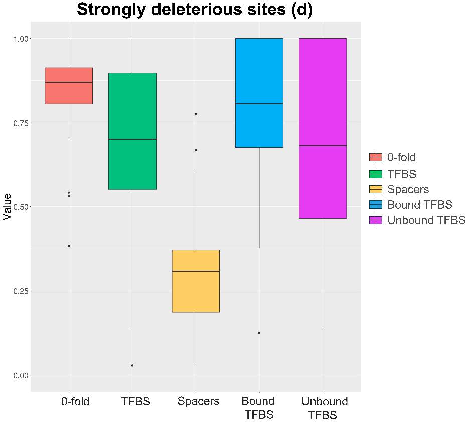
Figure 9. Strongly deleterious sites boxplot. Results obtained through generalized McDonald and Kreitman Test46
So, regarding the strongly deleterious fraction (figure 9) we can observe significant difference between some features and the spacers, which seem to have a lower proportion of strongly deleterious substitutions. In addition, this value is consistent with the other substitution proportions (figure 10 and figure 11). Similarly, the ratio of substitutions types is consistent in the other studied categories. The differences were checked through the Student’s t-test, showing significant results between 0-fold and spacers (pvalue<0.05; pvalue=1,48E-09), spacers and TFBS (pvalue<0.05; pvalue=1,468E-02), and spacers and Bound TFBS (pvalue<0.05; pvalue=3,398E-03), although there were not significant differences between spacers and Unbound TFBS (Anexo pvalues).
Moreover, spacers sequence seems to be the only category which have a remarkable proportion of neutral sites (figure 10). The differences between 0-fold and spacers (pvalue<0.05; pvalue=7,89E-03), TFBS and spacers (pvalue<0.05; pvalue=2,04E-02) and Spacers and Unbound TFBS (pvalue<0.05; pvalue=3,11E-02) were significant too. Consider CRM could be at intergenic and intronic regions, it would be legitimate to think that as other specific sequences at these areas, such as short intronic sequences, tend to evolve under neutrality. For that reason, the proportion of neutral substitutions are higher at spacers sequences [ref intrones]. It could seem contradictory, due to the fact that a given TFBS turn-over needs to occur at these sequences. However, spacers sequence as we explained before are so longer in comparison with TFBS motif, so they cannot be as the same constraints levels as TFBS motif. Therefore, in order to check this feature, we consider interesting to differentiate or classify in three categories the spacers sequence at next analyses, regarding their total size and the distance to TFBS motif. In this way, we could check if proximal TFBS motif instances are more constrained that distal, if TFBS turn-over tends to occur at proximal TFBS motif instances or not, and elucidate more detailed the behaviour in these sequences. In addition, significant results of the Student t-test were checked at the other variables, showing a significant lower proportion of neutral substitution between 0-fold selected sites and other variables (anexos).
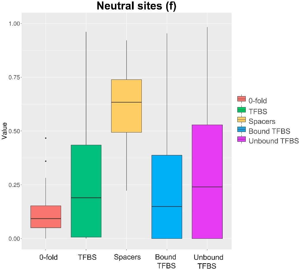
Figure 10. Neutral sites boxplot. Results obtained through generalized McDonald and Kreitman Test [ref]
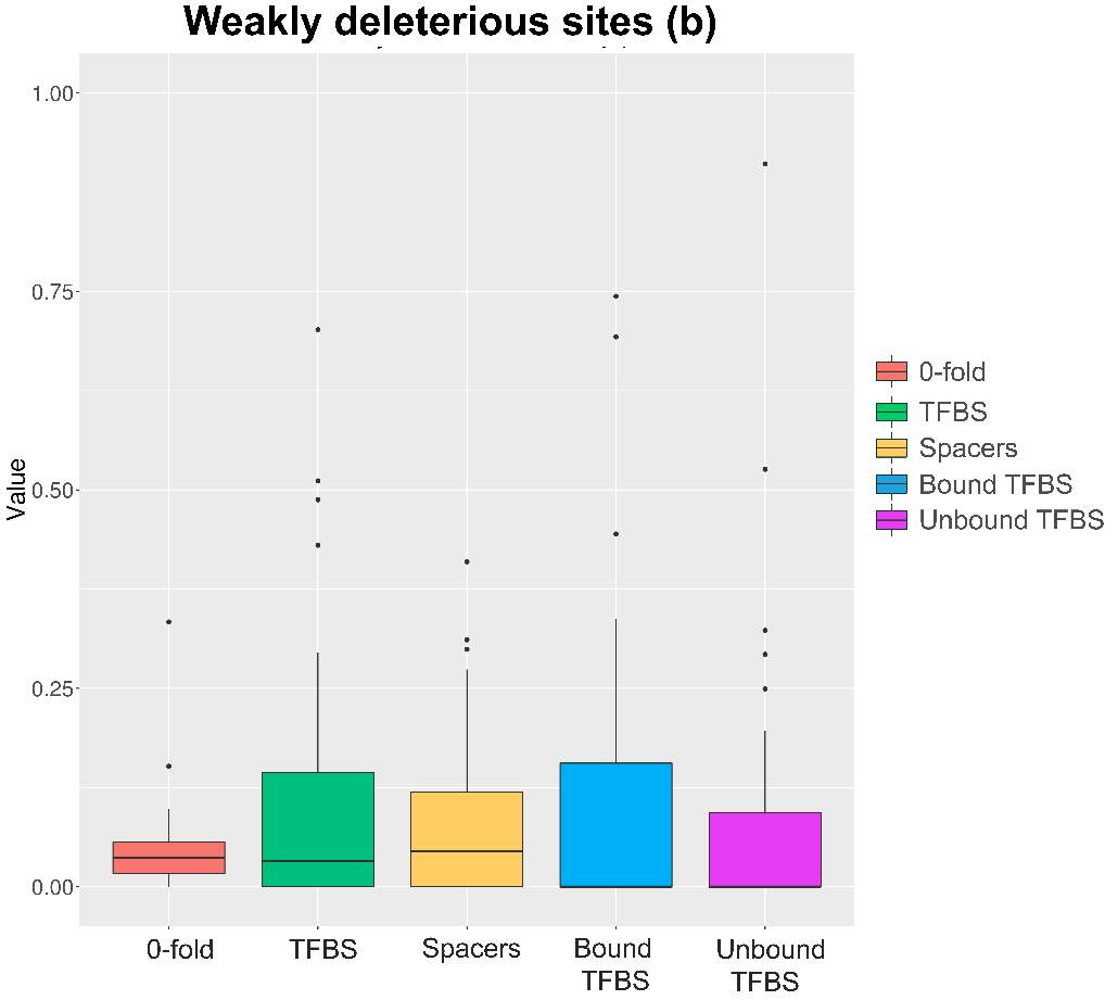
Figure 11. Weakly deleterious sites boxplot. Results obtained through generalized McDonald and Kreitman Test [ref]
Weakly deleterious sites show multiple significant results (anexo), although the overall mean of Bound and Unbound is near 0. It is due mainly the transformation of negative values into 0. These negative values are mainly due to the low or absence values of segregating and/or divergent sites at the selected TFBS positions. In order to remove possible biases, negative values were considered 0.
Regarding the fraction of adaptive fixations (anexos), there weren’t checked statistical differences among the variables measured. In this way, as we cannot check any significance difference we decide to execute a Fisher Exact Test to test what values are significant. Fisher Exact Test where execute on proper contingency tables necessaries to perform the MKT. At this manner, we decided to plot all the pvalues of our test in violins plots, in order to observe the pvalues distribution (figure 13). We could check that only 0-fold, and spacers contingency values has a significant number of pvalues, conversely the vast majority of pvalues at TFBS, Bound TFBS and Unbound TFBS tends to be 1. Again, the main reason whereby these contingency table, and then the final fraction of adaptive fixation, are not statistical significant is due to the low or absence number of segregating and/or divergence sites. In addition, we could check that TFBS have more pvalues distributed at the significant area than Bound or Unbound TFBS. If TFBS category have low values of segregating or divergent sites, Bound and Unbound TFBS values will lower indeed. In this way we need to say that the total number of TFBS selected as well as the total number target gene are not sufficiently high to include adequate numbers of segregating sites and/or divergent sites, thus, we are introducing biases impossible to control.
At the same way, the standard MKT were performed. At is expected the maintenance of the slightly deleterious mutation caused lower values at the fraction of adaptive fixation (figura anexo). Moreover, there weren’t significant differences among the variables. DoS were checked in order to test the aggregated pattern of selection across the different classes. Again, there weren’t statistical differences among the variables and any remarkable pattern (figura anexo).
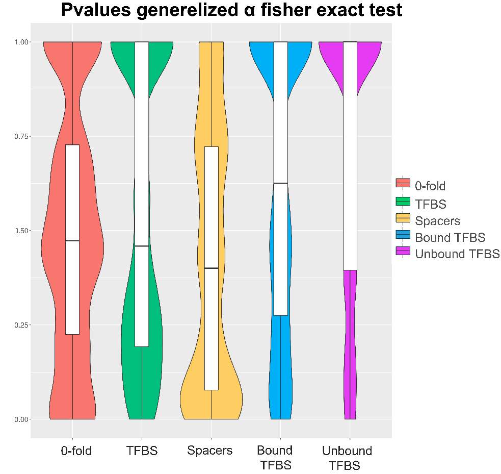
Figure12. Violin plots pvalues generalized α fisher exact test
So, through the multiple steps necessaries to execute the standard and generalized MKT we estimated the Nucleotide Diversity (π) and Divergence corrected by Jukes-Cantor (K). In this case the main component showing statistical difference among the variables were the 0fold sites (pvalues are shown at anexo x). At the same way, statistical differences at K are just showed between spacers and Bound TFBS (pvalues are shown at anexo). In addition to extend the information provide by these estimators we try to infer the correlation of π and K between 0-fold sites, TFBS and spacers and 4-fold sites (that would be expected to be the neutrally selected). So, we performed Pearson correlations test. As it would be expected 0-fold sites and 4-fold sites are significantly correlated (figure 15) in terms of divergence (pvalue= 1,10E-04; correlation=0.87). Because we cannot observe the same expectable pattern on the correlation between π 4-fold and π 0-fold, again, we need to assume that the statistical power would be insufficient, considering we were just checking the correlation between 36 values. We just observe another two-significant correlation although the correlation per se it so low; π TFBS ~ π 4fold (figura anexo): pvalue = 1,42E-04; correlation = 0.3, and K Spacers ~ K 4-fold (figura anexo): pvalue = 2,92E-02; correlation = 0.10).
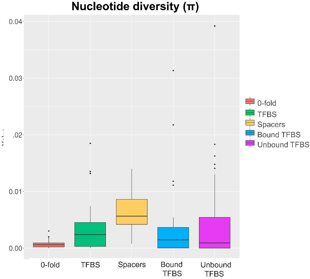
Figure 13. π values on the different categories
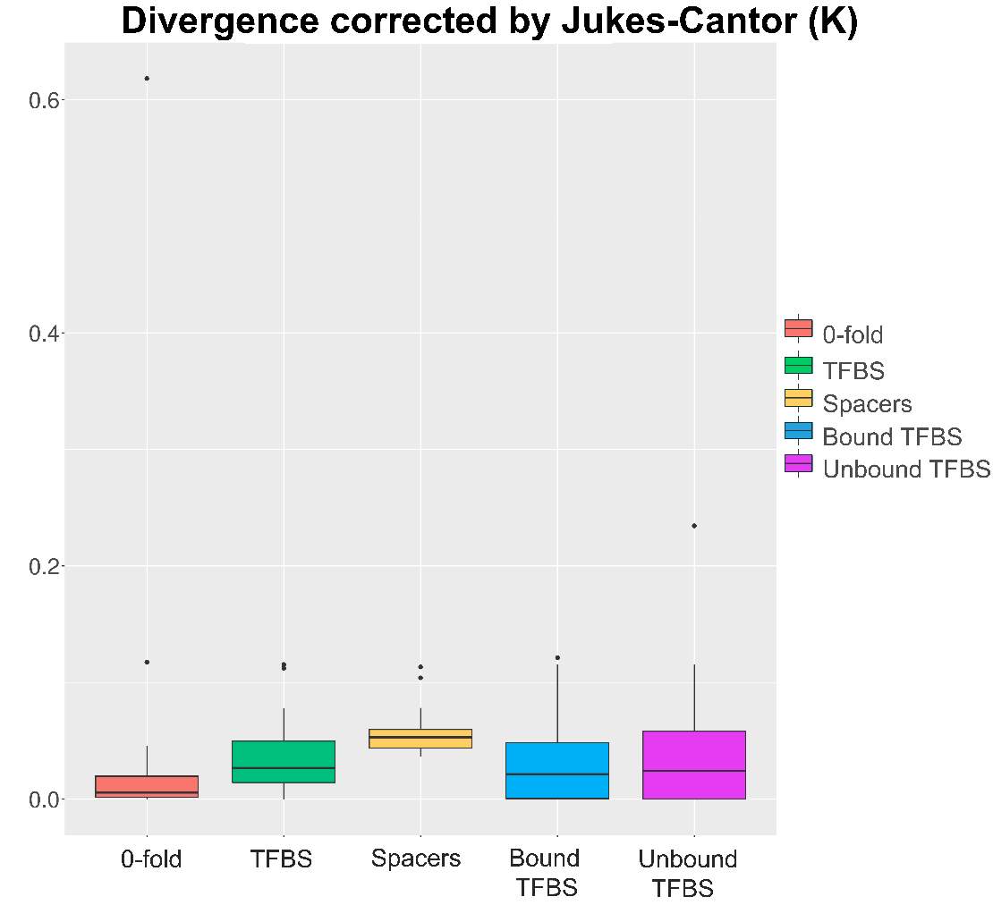
Figure 14. K values on the different categories.
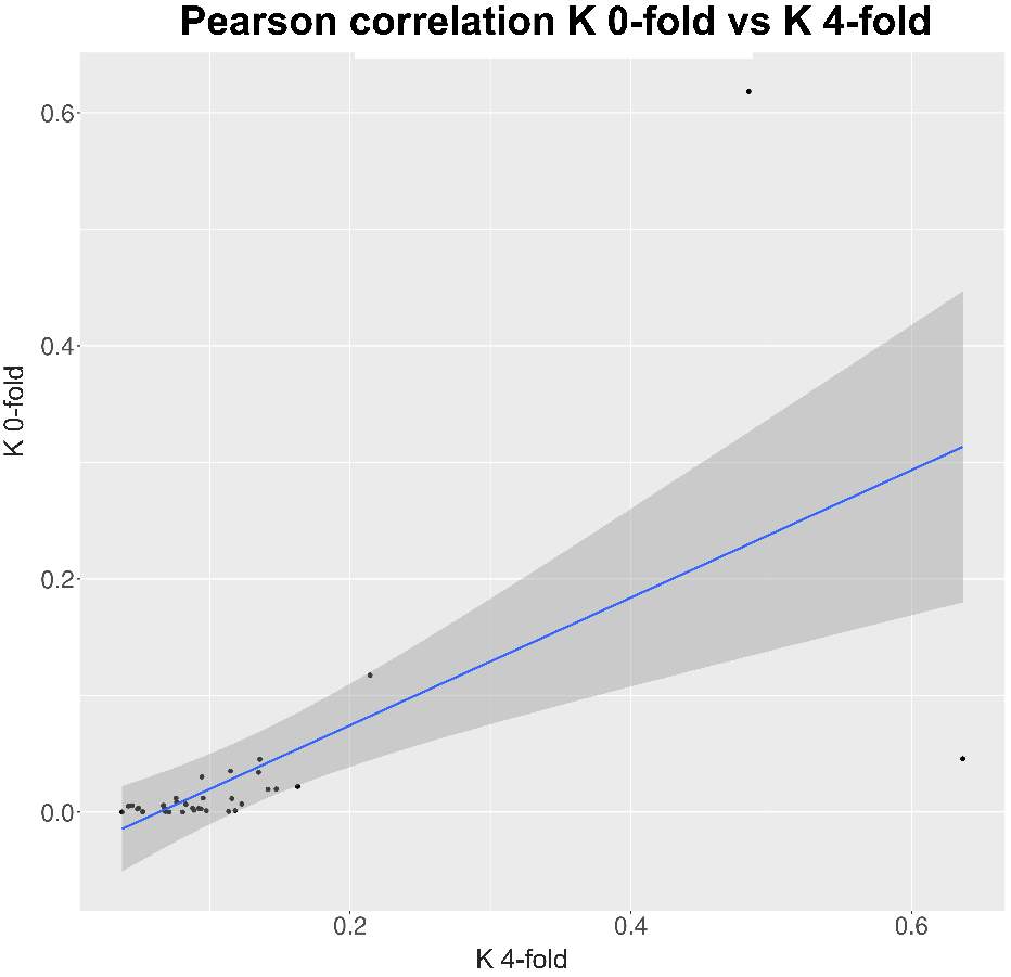
Figure 15. Correlation between K at 0-fold sites and K at 4-fold sites
In neither case there were significant differences between the Bound and Unbound TFBS. As we explained before, the differentiation between the two TFBS categories couldn’t be perform with the correct data due to his absence. In this way is normal to do not find any significant differences between them, due to a higher mutation rate at TFBS bound couldn’t be observe at this kind of ChIP-seq data.
5 Conclusion
Although the final results there weren’t highly relevant and the lack of the proper data is a problem to perform correctly the analysis, we decided to test a complete pipeline to execute the pertinent calculations. In this way, our pipeline allows to infer all the regulatory elements information regarding a target gene. This fact could be highly interesting in order to combine or extend the analysis to determined regulatory networks, specific recombination regions or particular development states. In addition, we consider very interesting extend our analysis to other Drosophila populations.
Due to pipeline were developed in a modular way, to extend or modify to other Drosophila population or specific developmental stages, would be easy. That it’s to say, that all the calculated parameters, the previous cleaning up steps and intermediates routines were developed independently. In this way, we achieved a scripts battery enough robust to replicate the completely the analysis and/or expand it, having created even dedicated functions in python and bash languages that could be useful to other kind of approaches. Nevertheless, the pipeline presents some bottlenecks. The most important concerns the intersection file through GenomicRanges Bioconductor library. Although through a user friendly Graphical User Interface (GUI) as Rstudio the performance is enough good, due to the R language limitations, the performance in a widely analysis is lesser, and moreover, the command line incorporation is more difficult. In this way tested the incorporation of some bash tools (such as BEDtools or Bedops) in order to improve our pipeline.
6 Appendix
Appendix I. Student’s t-test pvalues
| 0FOLD/SPACERS | 0FOLD/TFBS | 0FOLD/BOUND | 0FOLD/UNBOUND | SPACERS/TFBS | |
| P-value generalized α | 0,62341244 | 0,794940648 | 0,504690241 | 0,318305641 | 0,543011895 |
| P-value d | 1,48047E-09 | 0,014234759 | 0,114538749 | 0,00658823 | 0,014684005 |
| P-value b | 0,007891575 | 0,002734753 | 0,025445798 | 0,014379741 | 0,020350908 |
| P-value f | 2,44312E-05 | 0,042701716 | 0,163777003 | 0,038523183 | 0,029414036 |
| P-value standard α | 0,446272751 | 0,758454078 | 0,80130442 | 0,761267401 | 0,426900646 |
| P-value DoS | 0,343296446 | 0,771518445 | 0,826043348 | 0,982730158 | 0,17460349 |
| P-value π | 8,92E-12 | 0,001186114 | 0,01429242 | 0,007234085 | 0,003390191 |
| P-value K | 0,176440984 | 0,858703423 | 0,959774752 | 0,737655997 | 0,00070527 |
| SPACERS/BOUND | SPACERS/UNBOUND | TFBS/BOUND | TFBS/UNBOUND | BOUND/UNBOUND | |
| P-value generalized α | 0,400936654 | 0,264665515 | 0,62036849 | 0,350961566 | 0,318505431 |
| P-value d | 0,003397734 | 0,78850768 | 0,539536023 | 0,199646867 | 0,092131782 |
| P-value b | 0,118359804 | 0,03107079 | 0,585152757 | 0,349438917 | 0,200300974 |
| P-value f | 0,007580049 | 0,554527959 | 0,590940275 | 0,341530568 | 0,194666591 |
| P-value standard α | 0,322719507 | 0,541511352 | 0,921567306 | 0,983160891 | 0,915272568 |
| P-value DoS | 0,47246865 | 0,291935903 | 0,598881012 | 0,777614038 | 0,800011106 |
| P-value π | 0,046844353 | 0,342602493 | 0,847514352 | 0,393884357 | 0,541042227 |
| P-value K | 0,000202386 | 0,049784187 | 0,583507817 | 0,740800321 | 0,462641448 |
Appendix II. Data results
| ID | 0-fold d | 0-fold b | 0-fold f | 0-fold γ | 0-fold generalized α | TFBS d | TFBS b | TFBS f | TFBS γ | TFBS α |
| FBgn0000137 | NA | NA | NA | NA | -1 | NA | NA | NA | NA | NA |
| FBgn0000422 | 0,882860041 | 0,014642495 | 0,102497465 | 0,102497465 | -Inf | -0,472379603 | 0,511242918 | 0,961136686 | -0,001826939 | 0,034821429 |
| FBgn0000490 | 0,915577889 | -0,005628141 | 0,090050251 | -0,025070809 | 0,217777778 | 0,568939905 | 0,059743417 | 0,371316678 | 0,004055726 | -0,263391813 |
| FBgn0000576 | 0,859574468 | 0,056170213 | 0,084255319 | 0,039910414 | -0,9 | 912 | -0,0088 | 0,0088 | 0,000386191 | -Inf |
| FBgn0000606 | 0,969083548 | 0,003567283 | 0,027349169 | -0,667186212 | 0,960622353 | 0,883365732 | 0,001794373 | 0,114839895 | 0,007365393 | -0,56418832 |
| FBgn0001077 | 0,867924528 | 0,076310273 | 0,055765199 | -0,090533785 | 0,61882716 | 0,454545455 | 0,096969697 | 0,448484848 | -0,261856031 | 0,616885703 |
| FBgn0001168 | 0,93075616 | 0,020982982 | 0,048260858 | 0,025179578 | -1,090909091 | 0,406631248 | 0,104969411 | 0,488399342 | 0,017635935 | -1,537878788 |
| FBgn0001180 | 0,533009034 | 0 | 0,466990966 | 0,459915345 | -65 | -0,253731343 | 0,487562189 | 0,766169154 | 0,034026402 | -1,520833333 |
| FBgn0001319 | 0,91287012 | 0,022065359 | 0,065064521 | -0,037624266 | 0,366391185 | 0,6067908 | 0,268097182 | 0,125112018 | -0,007361627 | 0,884297521 |
| FBgn0001320 | 0,542274939 | 0,098083942 | 0,359641119 | 0,083137817 | -0,300675676 | 0,25862069 | -0,123563218 | 0,864942529 | 0,058975654 | -4,568181818 |
| FBgn0001325 | 0,784159882 | 0,035973353 | 0,179866765 | 0,081939304 | -0,836734694 | 0,717770035 | 0 | 0 | -0,011442294 | 1 |
| FBgn0002576 | 0,840067043 | 0,013181288 | 0,146751669 | 0,067546776 | -0,852810651 | 1 | 0 | 0 | -0,013992437 | 1 |
| FBgn0002973 | 0,903108899 | 0,020133216 | 0,076757885 | 0,076757885 | -Inf | 1 | 0 | 0 | 0 | NA |
| FBgn0003023 | 0,723238381 | 0,053223388 | 0,223538231 | -0,172166091 | 0,435087719 | 0,139393939 | 0,43030303 | 0,43030303 | 0,055389592 | -8,2 |
| FBgn0003448 | 0,712149533 | 0,151775701 | 0,136074766 | 0,098691589 | -2,64 | 0,795833333 | 0,163333333 | 0,040833333 | -0,01309816 | 0,813333333 |
| FBgn0003720 | 0,958381061 | 0,029480081 | 0,012138857 | -0,003468245 | 0,222222222 | 0,383230453 | 0,142511145 | 0,474258402 | -0,021526009 | 0,248148148 |
| FBgn0003884 | 1 | 0 | 0 | 0 | NA | 0,646875 | 0,08828125 | 0,26484375 | -0,230733463 | 0,7890625 |
| FBgn0003944 | 0,885287267 | 0,010925022 | 0,103787711 | 0,103787711 | -Inf | -0,331629709 | -0,111355794 | 1,442985503 | -0,013056489 | 0,134508349 |
| FBgn0003996 | 0,872595095 | 0,067177132 | 0,060227773 | -0,209071222 | 0,776353517 | 1 | 0 | 0 | -0,003954044 | 1 |
| FBgn0004045 | 0,928554502 | 0,057156398 | 0,0142891 | -0,050661353 | 0,78 | 0,705494505 | 0,088351648 | 0,206153846 | -0,128372866 | 692 |
| FBgn0004053 | 0,384313725 | 0,333496732 | 0,282189542 | 0,128267974 | -0,833333333 | 0,676954733 | 0,053840878 | 0,26920439 | 0,026410968 | -0,666666667 |
| FBgn0004170 | NA | NA | NA | NA | 0,410714286 | NA | NA | NA | NA | -3,8125 |
| FBgn0004197 | 0,897799043 | 0,029111788 | 0,073089169 | -0,028191058 | 0,278347107 | 0,029090909 | -0,093308146 | 1,064217237 | 0,001098938 | -0,032330579 |
| FBgn0004198 | 0,705502557 | 0,054586483 | 0,23991096 | -0,01598408 | 0,062463423 | -2,121263158 | -2,135601108 | 2,135601108 | 0,04775264 | -1,835872576 |
| FBgn0004837 | 0,97332782 | 0,015689518 | 0,010982662 | -0,019245809 | 0,636678201 | 0,578431373 | 0,247981546 | 0,173587082 | 0,005712189 | -Inf |
| FBgn0004862 | 0,861471861 | 0,029384757 | 0,109143382 | -0,111242293 | 0,504761905 | 0,701213819 | -0,039838157 | 0,338624339 | 0,000832319 | -0,079365079 |
| FBgn0004870 | 0,913372643 | 0,029680374 | 0,056946983 | -0,095924823 | 0,62748538 | 0,653367289 | 0,053515226 | 0,293117485 | -0,004504128 | 0,06042885 |
| FBgn0005613 | 0,865811634 | 0,039176833 | 0,095011533 | 0,024895089 | -0,355053508 | 1 | 0 | 0 | 0 | NA |
| FBgn0010382 | 0,804060018 | 0,041791395 | 0,154148588 | -0,004110629 | 0,025974026 | 0,79406308 | -0,074886153 | 0,074886153 | -0,000740041 | 0,757575758 |
| FBgn0010433 | 0,810286678 | 0,079047218 | 0,110666105 | -0,015809444 | 125 | 1 | 0 | 0 | 0 | NA |
| FBgn0011656 | 0,832830026 | -0,037613244 | 0,204783218 | 0,081334622 | -0,658854167 | -0,417682927 | 0,29535061 | 1,122332317 | 0,031806204 | -Inf |
| FBgn0011656 | 0,832830026 | -0,037613244 | 0,204783218 | 0,081334622 | -0,658854167 | -0,417682927 | 0,29535061 | 1,122332317 | 0,031806204 | -Inf |
| FBgn0015524 | 0,825471698 | 0,067629717 | 0,106898585 | 0,106898585 | -Inf | 0,723880597 | 0,120802239 | 0,155317164 | 0,020063464 | -Inf |
| FBgn0015904 | 0,770963705 | 0,037862998 | 0,191173297 | -0,005745265 | 0,029175841 | 1 | 0 | 0 | -0,010772627 | 1 |
| FBgn0086680 | 0,937725632 | 0,037364621 | 0,024909747 | -0,037364621 | 0,6 | -1,631355932 | 0,701694915 | 1,929661017 | 0,029579423 | -2,96 |
| FBgn0260642 | 1 | 0 | 0 | 0 | NA | 0,534904014 | -0,095404305 | 0,560500291 | -0,044286824 | 0,497863248 |
| FBgn0261648 | 0,90962348 | 0,045754799 | 0,044621721 | -0,231745042 | 0,838541654 | 0,666757123 | 0,010658088 | 0,322584789 | -0,001274546 | 0,071927457 |
| ID | Spacers d | Spacers b | Spacers f | Spacers γ | Spacers generalized α | 0 fold fisher exact test | TFBS fisher exact test | Spacers fisher exact test | 0-fold standard α | 0 fold standard α fisher exact test |
| FBgn0000137 | NA | NA | NA | NA | -0,445652174 | 0,654589372 | 1 | 1 | -1 | 0,654589372 |
| FBgn0000422 | -0,051567164 | 0,015083955 | 1,032173507 | 0,56297818 | -1,199880192 | 0,009453782 | 1 | 0,062172575 | -Inf | 0,009453782 |
| FBgn0000490 | 0,324267723 | -0,038392529 | 0,714124805 | -0,058210119 | 0,07536901 | 0,722475028 | 0,630965389 | 1 | 0,266666667 | 0,722475028 |
| FBgn0000576 | 0,21217086 | 0,26106495 | 0,52676419 | 0,06740045 | -0,146725664 | 0,47834325 | 1 | 0,731823694 | -2,166666667 | 0,193797313 |
| FBgn0000606 | 0,776845058 | 0,000446693 | 0,22270825 | 0,152514792 | -2,172777875 | 6,79E-07 | 0,26453553 | 9,70E-05 | 0,955486138 | 6,79E-07 |
| FBgn0001077 | 0,37697198 | 0,123616671 | 0,494466682 | -0,405843039 | 0,45078158 | 0,42501888 | 0,057363811 | 0,221482451 | 0,097222222 | 1 |
| FBgn0001168 | 0,090229002 | 0,039963203 | 0,869807795 | 0,287821936 | -0,494551426 | 1 | 0,106739968 | 0,384816633 | -2 | 0,59826087 |
| FBgn0001180 | -0,158762131 | 0,107672587 | 1,051089544 | 0,676333006 | -1,804726368 | 1,01E-06 | 0,165487895 | 0,026792105 | -65 | 1,01E-06 |
| FBgn0001319 | -0,015629348 | 0,094600349 | 0,921028999 | -0,059219819 | 0,060413048 | 0,509503437 | 0,166827689 | 0,869792471 | 0,151515152 | 1 |
| FBgn0001320 | -0,057747421 | 0,056481658 | 1,001265762 | 0,71020184 | -2,440020161 | 0,740930372 | 0,025642517 | 0,012990712 | -0,655405405 | 0,528707234 |
| FBgn0001325 | 0,068270337 | 0,29913426 | 0,632595403 | -0,189342724 | 0,230361286 | 0,468370761 | 0,292832492 | 0,627993312 | -1,204081633 | 0,300532913 |
| FBgn0002576 | 0,669025059 | -0,001552415 | 0,332527356 | -0,353102033 | 0,515004227 | 0,377452485 | 0,380952381 | 0,062803527 | -1,019230769 | 0,369916857 |
| FBgn0002973 | -0,129515217 | 0,060762078 | 1,068753139 | -0,228953829 | 0,176429529 | 0,152291573 | 1 | 0,719583312 | -Inf | 0,079129515 |
| FBgn0003023 | 0,502844639 | 0,12428884 | 0,372866521 | 0,068899248 | -0,226666667 | 0,226902691 | 0,201269604 | 0,781229534 | 0,300584795 | 0,496726947 |
| FBgn0003448 | 0,075613497 | 0,311134969 | 0,613251534 | 0,194539877 | -0,464615385 | 0,219972809 | 0,273504274 | 0,512091039 | -6,7 | 0,016516359 |
| FBgn0003720 | 0,271328523 | 0,235661609 | 0,493009868 | -0,044819079 | 0,083333333 | 1 | 0,635160976 | 0,862909758 | -1,666666667 | 0,635332336 |
| FBgn0003884 | 0,013100437 | 0,164483261 | 0,822416303 | 0,146207343 | -0,216216216 | 1 | 0,363411995 | 1 | NA | 1 |
| FBgn0003944 | -0,100526967 | -0,160864951 | 1,260446448 | 0,117688492 | -0,102986368 | 0,25 | 1 | 1 | -Inf | 0,25 |
| FBgn0003996 | 0,083380661 | 0,061663483 | 0,854955856 | 0,399252261 | -0,876122694 | 0,035166607 | 1 | 0,074586732 | 0,52690167 | 0,280489043 |
| FBgn0004045 | 0,306192893 | 0,044893401 | 0,648913706 | -0,853716659 | 0,568148148 | 0,604347826 | 0,276293305 | 0,122059485 | -0,1 | 1 |
| FBgn0004053 | -0,624274539 | 0,409370006 | 1,214904534 | 0,756485587 | -1,650205761 | 0,437551208 | 0,59705228 | 0,192144974 | -3 | 0,086082243 |
| FBgn0004170 | NA | NA | NA | NA | 0,658978175 | 1 | 0,146174259 | 0,079039979 | -0,178571429 | 1 |
| FBgn0004197 | 0,309433477 | -0,04110416 | 0,731670683 | 0,128903054 | -0,213851985 | 0,519486984 | 1 | 0,421263259 | -0,009090909 | 1 |
| FBgn0004198 | -1,233169966 | -0,496079862 | 2,713848655 | 2,421226384 | -8,274238227 | 1 | 0,067957075 | 1,87E-21 | -0,150852483 | 0,741468504 |
| FBgn0004837 | 0,160716206 | -0,019584649 | 0,858868443 | 0,009873927 | -0,011630142 | 0,602597403 | 1 | 1 | 0,117647059 | 1 |
| FBgn0004862 | 0,256905646 | 0,025968351 | 0,717126003 | -0,653203908 | 0,476676385 | 0,382349023 | 1 | 0,078286816 | 0,371428571 | 0,570678964 |
| FBgn0004870 | 0,602474394 | 0,101124935 | 0,296400671 | -0,175660986 | 0,372114497 | 0,02248792 | 1 | 0,247903562 | 0,433333333 | 0,173286903 |
| FBgn0005613 | 0,31657624 | 0,175790348 | 0,507633412 | 0,054501056 | -0,12027624 | 0,616677524 | 1 | 0,697279383 | -0,913793103 | 0,240155087 |
| FBgn0010382 | 0,366346915 | 0,044402487 | 0,589250598 | -0,091617131 | 0,134559367 | 1 | 0,410714286 | 0,678877175 | -0,238095238 | 0,672378031 |
| FBgn0010433 | 0,036417203 | 0,273926315 | 0,689656482 | 0,416713837 | -1,526745068 | 1 | 1 | 0,088357413 | -0,5 | 0,678925055 |
| FBgn0011656 | -0,0311906 | -0,169075082 | 1,200265682 | 0,425585031 | -0,549368351 | 0,715693766 | 0,039130435 | 0,376834989 | -0,354166667 | 0,720770663 |
| FBgn0011656 | -0,0311906 | -0,169075082 | 1,200265682 | 0,425585031 | -0,549368351 | 0,715693766 | 0,039130435 | 0,376834989 | -0,354166667 | 0,720770663 |
| FBgn0015524 | 0,366886247 | -0,001671955 | 0,634785709 | -0,310426374 | 0,328419811 | 0,155013263 | 1 | 0,498440131 | -Inf | 0,071953587 |
| FBgn0015904 | 0,308492404 | -0,101272944 | 0,79278054 | 0,485760673 | -1,582179931 | 1 | 0,506790123 | 0,000839791 | -0,163101604 | 0,733625501 |
| FBgn0086680 | -0,091240876 | -0,010792492 | 1,096037539 | 0,326572819 | -0,424415584 | 0,377318495 | 0,236381893 | 0,416092816 | NA | 1 |
| FBgn0260642 | 0,230207573 | 0,008553249 | 0,761239178 | -0,152247836 | 0,166666667 | 1 | 0,34272481 | 0,790522813 | NA | 1 |
| FBgn0261648 | 0,544946085 | 0,062919694 | 0,392134221 | 0,040863714 | -0,116331183 | 6,69E-09 | 1 | 0,582471413 | 0,672983398 | 4,93E-05 |
| ID | 0-fold DoS | TFBS standard α | TFBS standard α fisher exact test | TFBS DoS | Spacers standard α | Spacers standard α fisher exact test | Spacers DoS | |||
| FBgn0000137 | -0,166666667 | NA | 1 | 0 | -0,195652174 | 1 | -0,006578947 | |||
| FBgn0000422 | -0,333333333 | -0,478571429 | 0,474005977 | -0,088859416 | -1,241214058 | 0,061353816 | -0,036706349 | |||
| FBgn0000490 | 0,0625 | -0,466666667 | 0,467092106 | -0,083647799 | 0,125078699 | 0,843899129 | 0,001610045 | |||
| FBgn0000576 | -0,196969697 | -Inf | 1 | -0,047619048 | -0,715044248 | 0,117121228 | -0,05465368 | |||
| FBgn0000606 | 0,642257218 | -0,588628763 | 0,26453553 | -0,110275689 | -2,179141613 | 9,54E-05 | -0,087078279 | |||
| FBgn0001077 | 0,023809524 | 0,534050179 | 0,121916046 | 0,088782958 | 0,307984791 | 0,484489896 | 0,019565217 | |||
| FBgn0001168 | -0,130952381 | -2,083333333 | 0,053762172 | -0,249094203 | -0,563218391 | 0,379213265 | -0,006319298 | |||
| FBgn0001180 | -0,637254902 | -3125 | 0,028872188 | -0,333333333 | -2,092039801 | 0,011198536 | -0,090605473 | |||
| FBgn0001319 | 0,031347962 | 0,636363636 | 0,387127337 | 0,116666667 | -0,036093418 | 1 | -0,001108178 | |||
| FBgn0001320 | -0,122474747 | -3,772727273 | 0,051967243 | -0,360869565 | -2,634072581 | 0,012719541 | -0,086291734 | |||
| FBgn0001325 | -0,181538462 | -0,714285714 | 0,688923914 | -0,113636364 | -0,1335764 | 1 | -0,004556092 | |||
| FBgn0002576 | -0,139473684 | 1 | 0,380952381 | 0,0625 | 0,517268446 | 0,062803527 | 0,153684701 | |||
| FBgn0002973 | -0,24137931 | NA | 1 | 0 | 0,12960688 | 0,857045489 | 0,010921325 | |||
| FBgn0003023 | 0,084972723 | -17,4 | 0,033916569 | -0,155913978 | -0,635555556 | 0,428252087 | -0,115977291 | |||
| FBgn0003448 | -0,398809524 | 0,066666667 | 1 | 0,009803922 | -1,207692308 | 0,079859405 | -0,076985943 | |||
| FBgn0003720 | -0,084033613 | 0,022222222 | 1 | 0,005610098 | -0,35483871 | 0,378036529 | -0,034112934 | |||
| FBgn0003884 | 0 | 0,71875 | 0,363411995 | 0,270588235 | -0,459459459 | 0,760347242 | -0,077272727 | |||
| FBgn0003944 | -0,3 | 0,201298701 | 0,778042101 | 0,014821898 | 0,036955323 | 1 | 0,000219639 | |||
| FBgn0003996 | 0,1775 | 1 | 1 | 0,072727273 | -1,011437586 | 0,040735687 | -0,047476674 | |||
| FBgn0004045 | -0,016483516 | 0,56 | 0,310935661 | 0,19047619 | 0,538271605 | 0,1292294 | 0,10770751 | |||
| FBgn0004053 | -0,327272727 | -1 | 0,59705228 | -0,15 | -2,543209877 | 0,050625641 | -0,137700535 | |||
| FBgn0004170 | -0,03968254 | -3125 | 0,289796182 | -0,274725275 | 0,688988095 | 0,063670308 | 0,044214547 | |||
| FBgn0004197 | -0,001805986 | 0,058181818 | 1 | 0,012145749 | -0,145659604 | 0,568126065 | -0,013844495 | |||
| FBgn0004198 | -0,034983669 | -3,144736842 | 0,011196626 | -0,187598116 | -6,631578947 | 2,90E-17 | -0,384146341 | |||
| FBgn0004837 | 0,012383901 | -Inf | 0,49197861 | -0,105263158 | 0,011437908 | 1 | 0,001237186 | |||
| FBgn0004862 | 0,110795455 | 0,047619048 | 1 | 0,007692308 | 0,457725948 | 0,109911438 | 0,023732144 | |||
| FBgn0004870 | 0,115097856 | -0,111111111 | 1 | -0,00747443 | 0,157894737 | 0,710204679 | 0,037037037 | |||
| FBgn0005613 | -0,128143133 | NA | 1 | 0 | -0,508221055 | 0,121548385 | -0,034015009 | |||
| FBgn0010382 | -0,051789077 | 0,333333333 | 1 | 0,014066496 | 0,069344811 | 0,889706032 | 0,002205128 | |||
| FBgn0010433 | -0,095238095 | NA | 1 | 0 | -2,530349014 | 0,013833789 | -0,022937752 | |||
| FBgn0011656 | -0,068825911 | -Inf | 0,015942029 | -0,428571429 | -0,331117021 | 0,653014948 | -0,015293901 | |||
| FBgn0011656 | -0,068825911 | -Inf | 0,015942029 | -0,428571429 | -0,331117021 | 0,653014948 | -0,015293901 | |||
| FBgn0015524 | -0,384615385 | -Inf | 0,294749695 | -0,2 | 0,330188679 | 0,498440131 | 0,052760505 | |||
| FBgn0015904 | -0,037240537 | 1 | 0,506790123 | 0,042553191 | -1,252321981 | 0,005132918 | -0,181634486 | |||
| FBgn0086680 | NA | -Inf | 0,075 | -0,948717949 | -Inf | 1,81E-05 | -185 | |||
| FBgn0260642 | 0 | 0,583333333 | 0,187173621 | 0,154499151 | 0,157303371 | 0,79138831 | 0,003356777 | |||
| FBgn0261648 | 0,261195001 | 0,041264267 | 1 | 0,006107862 | -0,295451526 | 0,171693482 | -0,036368097 |
Appendix III. Figures
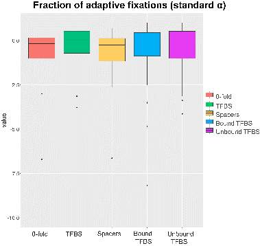
Figure 1. Standard α values
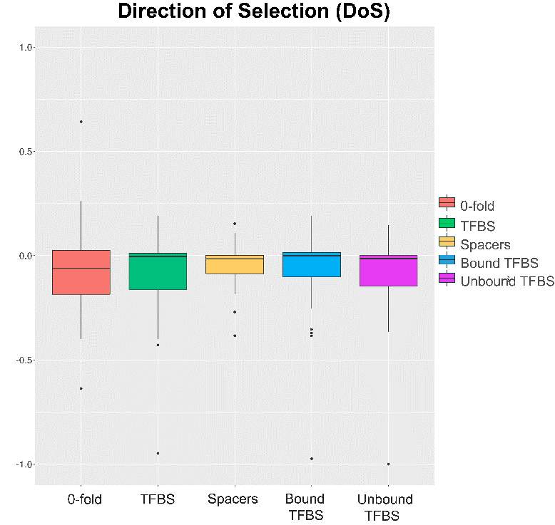
Figure 2. Direction of Selection
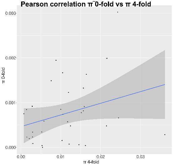
Figure 3. π 0-fold ~ π 4-fold Pearson correlation
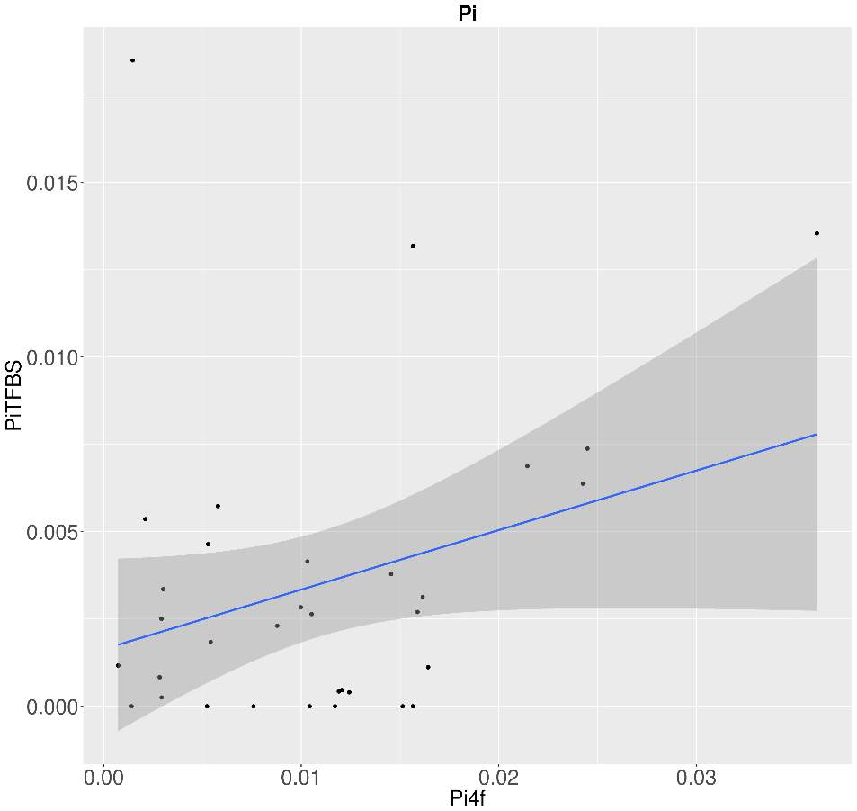
Figure 4. π TFBS ~ π 4-fold Pearson correlation
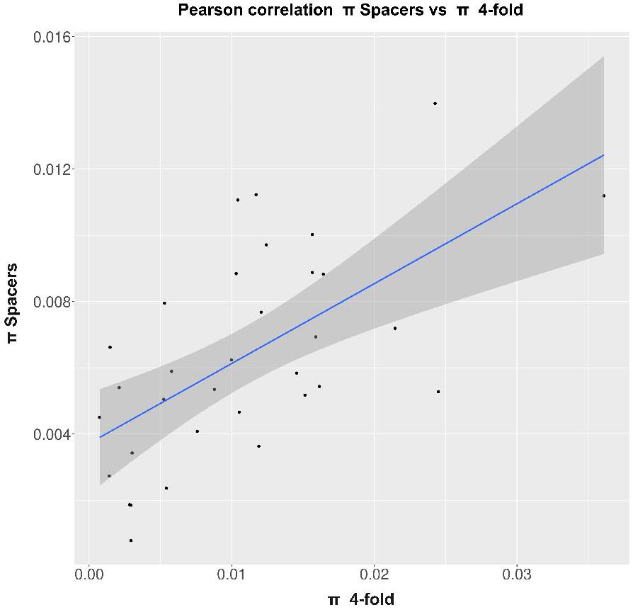
Figure 5. π Spacers~ π 4-fold Pearson correlation
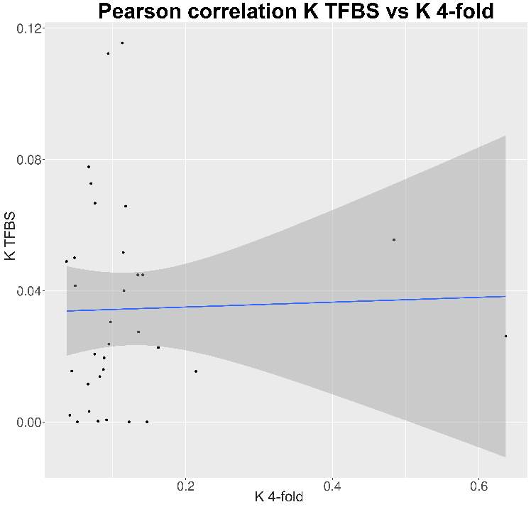
Figure 6. K TFBS~ K 4-fold Pearson correlation
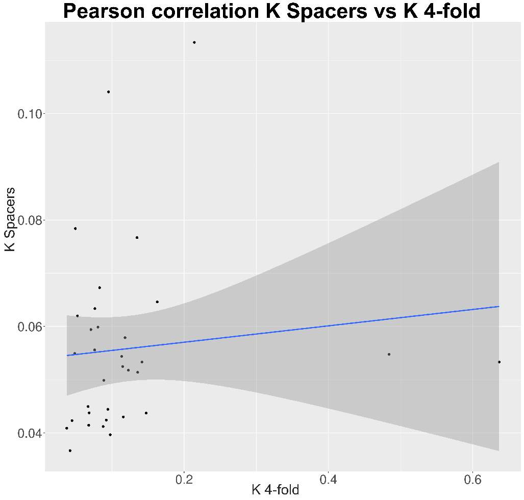
Figure 7. K Spacers~ K 4-fold Pearson correlation
7 Bibliography
1. Davies, J. & Jacob, F. Genetic mapping of the regulator and operator genes of the lac operon. J. Mol. Biol. 36, 413–417 (1968).
2. Jeziorska, D. M., Jordan, K. W. & Vance, K. W. A systems biology approach to understanding cis-regulatory module function. Semin. Cell Dev. Biol. 20, 856–862 (2009).
3. Suryamohan, K. & Halfon, M. S. Identifying transcriptional cis -regulatory modules in animal genomes: Identifying transcriptional cis -regulatory modules. Wiley Interdiscip. Rev. Dev. Biol. 4, 59–84 (2015).
4. Spitz, F. & Furlong, E. E. M. Transcription factors: from enhancer binding to developmental control. Nat. Rev. Genet. 13, 613–626 (2012).
5. Swanson, C. I., Evans, N. C. & Barolo, S. Structural Rules and Complex Regulatory Circuitry Constrain Expression of a Notch- and EGFR-Regulated Eye Enhancer. Dev. Cell 18, 359–370 (2010).
6. Rossi, F. M., Kringstein, A. M., Spicher, A., Guicherit, O. M. & Blau, H. M. Transcriptional control: rheostat converted to on/off switch. Mol. Cell 6, 723–728 (2000).
7. Arnosti, D. N. & Kulkarni, M. M. Transcriptional enhancers: Intelligent enhanceosomes or flexible billboards? J. Cell. Biochem. 94, 890–898 (2005).
8. Krejci, A., Bernard, F., Housden, B. E., Collins, S. & Bray, S. J. Direct Response to Notch Activation: Signaling Crosstalk and Incoherent Logic. Sci. Signal. 2, ra1-ra1 (2009).
9. Sandmann, T. et al. A Temporal Map of Transcription Factor Activity: Mef2 Directly Regulates Target Genes at All Stages of Muscle Development. Dev. Cell 10, 797–807 (2006).
10. Hong, J.-W., Hendrix, D. A. & Levine, M. S. Shadow Enhancers as a Source of Evolutionary Novelty. Science 321, 1314–1314 (2008).
11. Perry, M. W., Boettiger, A. N., Bothma, J. P. & Levine, M. Shadow Enhancers Foster Robustness of Drosophila Gastrulation. Curr. Biol. 20, 1562–1567 (2010).
12. Barolo, S. Shadow enhancers: Frequently asked questions about distributed cis-regulatory information and enhancer redundancy. BioEssays 34, 135–141 (2012).
13. Blackwood, E. M. Going the Distance: A Current View of Enhancer Action. Science 281, 60–63 (1998).
14. Würtele, H. & Chartrand, P. Genome-wide scanning of HoxB1-associated loci in mouse ES cells using an open-ended Chromosome Conformation Capture methodology. Chromosome Res. 14, 477–495 (2006).
15. Dostie, J. & Dekker, J. Mapping networks of physical interactions between genomic elements using 5C technology. Nat. Protoc. 2, 988–1002 (2007).
16. Sainsbury, S., Bernecky, C. & Cramer, P. Structural basis of transcription initiation by RNA polymerase II. Nat. Rev. Mol. Cell Biol. 16, 129–143 (2015).
17. Hardison, R. C. & Taylor, J. Genomic approaches towards finding cis-regulatory modules in animals. Nat. Rev. Genet. 13, 469–483 (2012).
18. Jing, H. et al. Exchange of GATA Factors Mediates Transitions in Looped Chromatin Organization at a Developmentally Regulated Gene Locus. Mol. Cell 29, 232–242 (2008).
19. Wasserman, W. W. & Fickett, J. W. Identification of regulatory regions which confer muscle-specific gene expression. J. Mol. Biol. 278, 167–181 (1998).
20. Wasserman, W. W. & Sandelin, A. Applied bioinformatics for the identification of regulatory elements. Nat. Rev. Genet. 5, 276–287 (2004).
21. Su, J., Teichmann, S. A. & Down, T. A. Assessing Computational Methods of Cis-Regulatory Module Prediction. PLoS Comput. Biol. 6, e1001020 (2010).
22. Smith, A. D., Sumazin, P., Xuan, Z. & Zhang, M. Q. DNA motifs in human and mouse proximal promoters predict tissue-specific expression. Proc. Natl. Acad. Sci. 103, 6275–6280 (2006).
23. Sinha, S. & He, X. MORPH: Probabilistic Alignment Combined with Hidden Markov Models of cis-Regulatory Modules. PLoS Comput. Biol. 3, e216 (2007).
24. Zhou, Q. & Wong, W. H. CisModule: De novo discovery of cis-regulatory modules by hierarchical mixture modeling. Proc. Natl. Acad. Sci. 101, 12114–12119 (2004).
25. Zhou, Q. & Wong, W. H. Coupling hidden Markov models for the discovery of Cis-regulatory modules in multiple species. Ann. Appl. Stat. 1, 36–65 (2007).
26. Kantorovitz, M. R. et al. Motif-Blind, Genome-Wide Discovery of cis-Regulatory Modules in Drosophila and Mouse. Dev. Cell 17, 568–579 (2009).
27. Ivan, A., Halfon, M. S. & Sinha, S. Computational discovery of cis-regulatory modules in Drosophila without prior knowledge of motifs. Genome Biol. 9, R22 (2008).
28. Ludwig, M. Z. et al. Functional Evolution of a cis-Regulatory Module. PLoS Biol. 3, e93 (2005).
29. Kheradpour, P., Stark, A., Roy, S. & Kellis, M. Reliable prediction of regulator targets using 12 Drosophila genomes. Genome Res. 17, 1919–1931 (2007).
30. Stark, A. et al. Discovery of functional elements in 12 Drosophila genomes using evolutionary signatures. Nature 450, 219–232 (2007).
31. He, B. Z., Holloway, A. K., Maerkl, S. J. & Kreitman, M. Does Positive Selection Drive Transcription Factor Binding Site Turnover? A Test with Drosophila Cis-Regulatory Modules. PLoS Genet. 7, e1002053 (2011).
32. Torgerson, D. G. et al. Evolutionary Processes Acting on Candidate cis-Regulatory Regions in Humans Inferred from Patterns of Polymorphism and Divergence. PLoS Genet. 5, e1000592 (2009).
33. Moses, A. M. et al. Large-Scale Turnover of Functional Transcription Factor Binding Sites in Drosophila. PLoS Comput. Biol. 2, e130 (2006).
34. Dermitzakis, E. T. & Clark, A. G. Evolution of transcription factor binding sites in Mammalian gene regulatory regions: conservation and turnover. Mol. Biol. Evol. 19, 1114–1121 (2002).
35. Su, J., Teichmann, S. A. & Down, T. A. Assessing Computational Methods of Cis-Regulatory Module Prediction. PLoS Comput. Biol. 6, e1001020 (2010).
36. Guo, H., Huo, H. & Yu, Q. SMCis: An Effective Algorithm for Discovery of Cis-Regulatory Modules. PLOS ONE 11, e0162968 (2016).
37. Zambelli, F., Pesole, G. & Pavesi, G. Motif discovery and transcription factor binding sites before and after the next-generation sequencing era. Brief. Bioinform. 14, 225–237 (2013).
38. Davidson, E. H. The regulatory genome: gene regulatory networks in development and evolution. (Elsevier, Acad. Press, 2006).
39. Boyle, A. P. et al. High-Resolution Mapping and Characterization of Open Chromatin across the Genome. Cell 132, 311–322 (2008).
40. de-Leon, S. B.-T. & Davidson, E. H. Gene Regulation: Gene Control Network in Development. Annu. Rev. Biophys. Biomol. Struct. 36, 191–212 (2007).
41. Megason, S. G. & Fraser, S. E. Digitizing life at the level of the cell: high-performance laser-scanning microscopy and image analysis for in toto imaging of development. Mech. Dev. 120, 1407–1420 (2003).
42. Andolfatto, P. Adaptive evolution of non-coding DNA in Drosophila. Nature 437, 1149–1152 (2005).
43. Ludwig, M. Functional evolution of noncoding DNA. Curr. Opin. Genet. Dev. 12, 634–639 (2002).
44. Arbiza, L. et al. Genome-wide inference of natural selection on human transcription factor binding sites. Nat. Genet. 45, 723–729 (2013).
45. Kimura, M. The role of compensatory neutral mutations in molecular evolution. J. Genet. 64, 7–19 (1985).
46. Rubinstein, M. & de Souza, F. S. J. Evolution of transcriptional enhancers and animal diversity. Philos. Trans. R. Soc. B Biol. Sci. 368, 20130017–20130017 (2013).
47. McDonald, J. H. & Kreitman, M. Adaptive protein evolution at the Adh locus in Drosophila. Nature 351, 652–654 (1991).
48. Bird, C. P., Stranger, B. E. & Dermitzakis, E. T. Functional variation and evolution of non-coding DNA. Curr. Opin. Genet. Dev. 16, 559–564 (2006).
49. Hare, E. E., Peterson, B. K., Iyer, V. N., Meier, R. & Eisen, M. B. Sepsid even-skipped enhancers are functionally conserved in Drosophila despite lack of sequence conservation. PLoS Genet. 4, e1000106 (2008).
50. Sabarinathan, R., Mularoni, L., Deu-Pons, J., Gonzalez-Perez, A. & López-Bigas, N. Nucleotide excision repair is impaired by binding of transcription factors to DNA. Nature 532, 264–267 (2016).
51. Mackay, T. F. C. et al. The Drosophila melanogaster Genetic Reference Panel. Nature 482, 173–178 (2012).
52. Hervas, S., Sanz, E., Casillas, S., Pool, J. E. & Barbadilla, A. PopFly: the Drosophila population genomics browser. Bioinformatics (2017). doi:10.1093/bioinformatics/btx301
53. Hu, T. T., Eisen, M. B., Thornton, K. R. & Andolfatto, P. A second-generation assembly of the Drosophila simulans genome provides new insights into patterns of lineage-specific divergence. Genome Res. 23, 89–98 (2013).
54. Gallo, S. M. et al. REDfly v3.0: toward a comprehensive database of transcriptional regulatory elements in Drosophila. Nucleic Acids Res. 39, D118–D123 (2011).
55. Hutter, S., Vilella, A. J. & Rozas, J. Genome-wide DNA polymorphism analyses using VariScan. BMC Bioinformatics 7, 409 (2006).
56. Egea, R., Casillas, S. & Barbadilla, A. Standard and generalized McDonald-Kreitman test: a website to detect selection by comparing different classes of DNA sites. Nucleic Acids Res. 36, W157–W162 (2008).
Cite This Work
To export a reference to this article please select a referencing stye below:
Related Services
View all


Related Content
All TagsContent relating to: "Biology"
Biology is the scientific study of the natural processes of living organisms or life in all its forms. including origin, growth, reproduction, structure, and behaviour and encompasses numerous fields such as botany, zoology, mycology, and microbiology.
Related Articles

DMCA / Removal Request
If you are the original writer of this dissertation and no longer wish to have your work published on the UKDiss.com website then please: