Integrating 4D Seismic Data and Production Data in Complex Reservoir Characterization
Info: 8026 words (32 pages) Dissertation
Published: 26th Nov 2021
Tagged: Engineering
Chapter One - Introduction
This chapter lays the foundation and sets out the framework of this thesis. First, the importance of integrating 4D seismic data and production data in resolving the challenges of complex reservoir characterization is demonstrated, using examples from the literature. Geomechanically active reservoirs and the associated challenges in seismic interpretation and analysis are also discussed. I also explore the literature on pressure-saturation estimation on chalk reservoirs and the proxy model solution. Finally, I provide an overview of the content of this thesis.
1.1 Preamble
Time-lapse seismic or 4D seismic is the investigation of seismic attribute changes by acquiring seismic data through different time periods during the production period of a field. The first repeated 3D seismic surveys were acquired in North Texas in 1982/1983 to monitor a combustion process around an injection well (Mohamed and Samsudin, 2011). Since this seismic study was performed as the first is sui generis, and it was ahead of its time, the results did not prove it to be an economic method. However, now, nearly forty years after its first beginnings, 4D seismic has become commonplace in oil and gas field development as a proven technology. For example, nearly 75% of today’s Statoil’s field had acquired 4D seismic surveys by the year 2009 (Sandø et al., 2009). Traditionally, time-lapse seismic was used to discover the “low hanging fruits”, such as identifying un-swept areas and by-passed oil, to target infill drilling wells and to improve our knowledge of the geological framework.
In recent years, combined with reservoir modelling, time-lapse seismic monitoring enables reservoir engineers to improve reservoir characterization and reduce uncertainty in production forecasts (Roggero et al., 2012). Pressure and saturation monitoring is key in field development, such as assessment of field connectivity, monitoring well performance, drilling infill wells, understanding injection and aquifer support and evaluating the average pressure state of the field (Corzo et al., 2013). The decomposition of pressure and saturation changes is also crucial to explain different physical variables that contributed to similar 4D seismic differences. The oil and gas industry is constantly pushing the boundaries of technology and ideas. Figure 1.1 shows the value chain of 4D seismic, demonstrating the vast contributions of 4D in different reservoir management and operations domains.
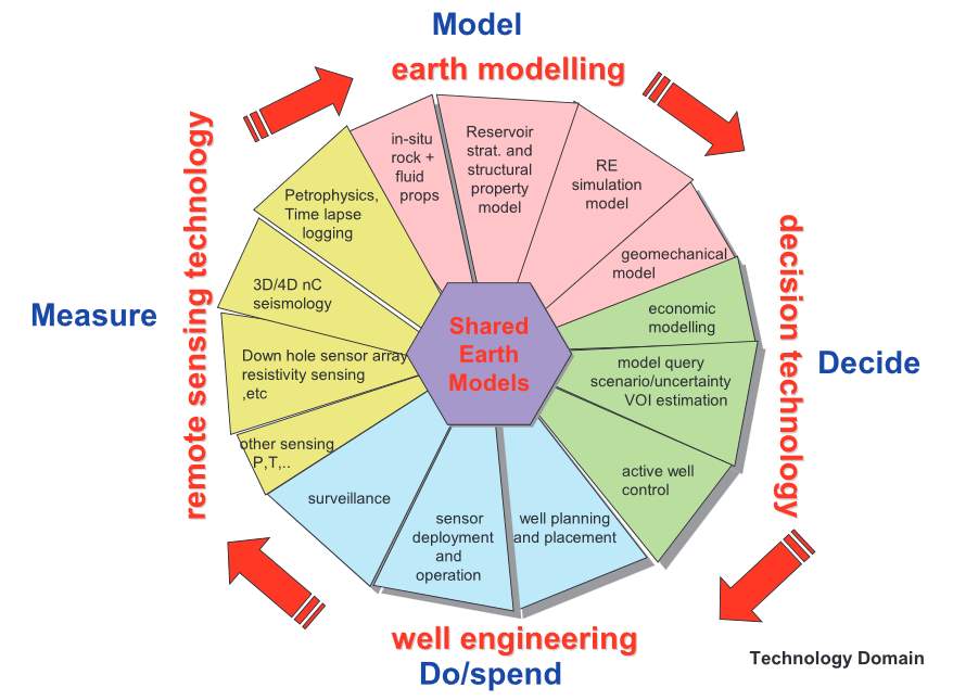
Figure 1.1: The 4D ‘Value Loop’ (de Waal and Calvert 2003).
An emerging technology known as the seismic permanent reservoir monitoring (PRM) system, is paving the way to delivering better quality and higher repeatability seismic data. In the past, the majority (in the range of 95%) of offshore seismic time-lapse surveys were acquired using towed streamer, but this is now changing. The PRM system has improved repeatability so much that the technology has claimed changes in travel time as small as a few hundred microseconds, and 2-3% changes in amplitude are detectable above noise level (Bertrand et al., 2014). Figure 1.2 illustrates the growth in offshore PRM use since the Foinaven installation, we can see an increase in the number of kilometers of installed seismic sensor cables versus the year of installation. The forecast does not specify field names. Higher detectability in time-lapse seismic change means better operational efficiency, lower reservoir management costs, reduction of overburden drilling risk, better monitoring of cap rock integrity and higher success rate in unravelling reservoir dynamic changes such as pressure and saturation (Caldwell et al., 2015).
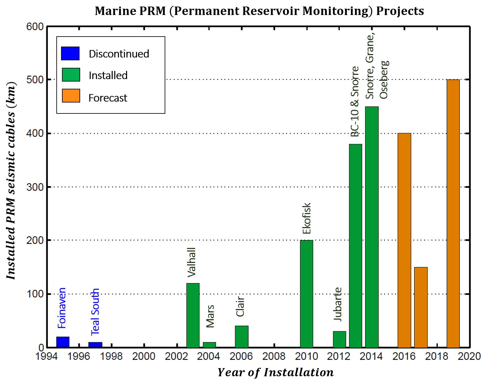
Figure 1.2: Summary of seabed PRM projects over the last 20 years and those forecasted for the future (Reproduced after Caldwell et al., 2015).
1.2 Integration of Time-lapse Seismic and Engineering data
The integration of seismic and engineering data has been mainly qualitative, such that anomalies are often inferred to be changes in oil, water, or gas saturation (Sønneland et al., 1996; Anderson et al., 1997; He et al., 1998), or semi-quantitative, in which the interpretation of reservoir performance has been aided by the visual comparison of maps and plots of seismic attributes with areal plots of the reservoir simulator output. As a result, the reservoir model can often be improved by updating the model in areas of misfit. Semi-quantitative integration of time-lapse seismic and production data can be found in Al-Najjar et al. (1999), Waggoner (2001), Staples et al. (2002), Marsh et al. (2003), Landa and Kumar (2011), Ayzenberg et al. (2013), Alerini et al. (2014), Ayzenberg and Liu (2014) and Tian et al. (2014). A review of these articles shows that the comparison of the 4D signature with the predicted output from a simulation model has been successful in locating dynamic barriers, varying fault transmissibility multipliers, altering aquifer connectivity, identifying injected water slumping, STOIIP adjustment, well planning and changes in production strategies.
To move towards more quantitative solutions, one would need to merge flow simulation and 4D seismic in an attempt to provide vastly improved forecasts of reservoir behaviour and make major improvements in geological reservoir models. These developments hold significant impact on the future of 4D within the industry. Other examples are from the “global inversion” scheme by El Ouair and Stronen (2006) and Lafet et al. (2009); constraining 4D inversion results to the stratigraphy constraints, which honours the reservoir zonation, expected production effects and rock-physics trends (Figure 1.3). Seismic inversion is by its nature ill-posed and there are non-unique solutions. In addition, the inherent errors in the 4D data, as well as the imperfect modelling process, will make the inversion unstable. Therefore, the key for a successful 4D inversion lies in collaboration among the disciplines.
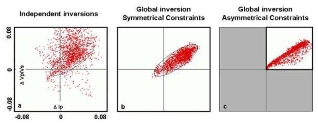
Figure 1.3: Inverted elastic attributes for a water flooded area by (a) independent inversion of baseline and monitor seismic data, (b) a global 4D inversion with a symmetrical searching window and (b) a non-symmetrical searching window as constraints (Lafet et al., 2009).
Quantitative examples such as that of Yin et al. (2015) have involved using well2seis attributes in seismic-assisted history matching to honour data from both seismic and engineering domains, and remaining consistent with fault interpretation. The well2seis attribute determines the correlation between production and seismic data across time. This promoted a 90% reduction in the misfit errors and 89% lowering of the corresponding uncertainty bounds after history matching with the well2seis attribute (Yin et al., 2015). Figure 1.4 shows that area ‘I’ shows a hardening signal due to pressure depletion, and this is not predicted in the simulation model in Figure 1.4 (b).
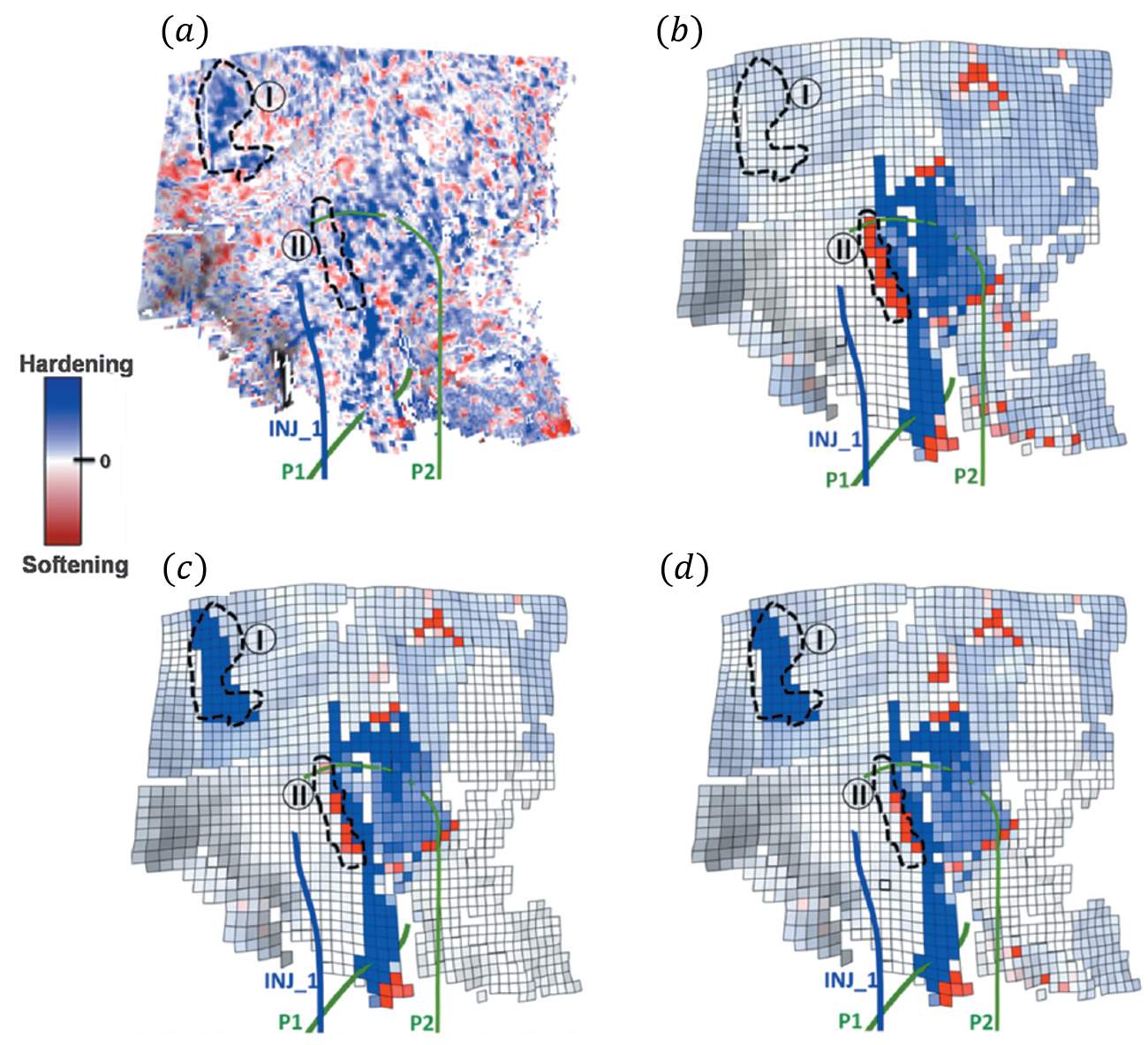
Figure 1.4: (a) Observed 4D seismic difference between baseline and monitor, (b) simulated 4D seismic difference from simulation model using traditional history matching without well2seis attribute, (c) simulated 4D seismic difference after direct updating and (d) the 4D difference after assisted history matching using well2seis (Yin et al., 2015).
1.3 Geomechanically Active Reservoirs
Reservoir compaction, subsidence and potential fault reactivation are notorious in depleting, weak, unconsolidated sandstone and chalk reservoirs. Reservoir compaction has been observed in a wide range of geographical locations and reservoir types, such as the North Sea, the Gulf of Mexico, California, Canada, South America and Southeast Asia (Bruno, 2002). It can be a positive phenomenon, because the compaction mechanism can provide significant energy to drive production, analogous to squeezing water from a sponge (Setarri, 2002). The value of the added production outweighs the negative effects of compaction, which are chalk production, well failures and damage on infrastructure (Barkved, 2012). The geomechanical challenges associated with a compacting reservoir are shown in Figure 1.5. Some of these challenges include slip planes in the overburden, well failure due to buckling-induced casing damage, a high shear zone in the overburden and a risk in seal integrity (Dusseault et al., 2001).
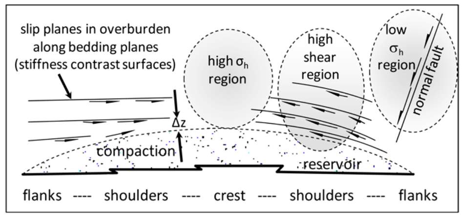
Figure 1.5: Geomechanical challenges both inside and outside the reservoir induced by production (Dusseault et al., 2001).
1.3.1 Challenges for time-lapse seismic analysis of a compacting reservoir
There are many challenges to interpret time lapse seismic signals from a compacting reservoir, due to the additional component of porosity reduction making interpretation more ambiguous. This is demonstrated in Figure 1.6: in the event of an injection event at high effective stress in a chalk reservoir, we have an interplay of (1) increase of water saturation, (2) pressure build up at injection point and (3) compaction due to weakening of the chalk. This results in complex behaviour such as cancellation in signals in the relative change of elastic properties and consequently amplitude changes and time-shifts.
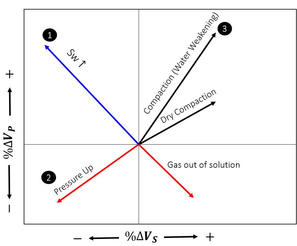
Figure 1.6: The behaviour of the relative change in P and S-wave velocity in an isolated event with different dynamic changes.
As the reservoir compacts, the immediate overburden stretches in response. Often the seabed produces subsidence, which means the seismic signal becomes time variant and cannot be exploited to match time-lapsed seismic surveys with each other. In the Valhall field, time-shifts up to 48ms have been measured from streamer 4D seismic data (Barkved et al., 2003). In order to discriminate between subsidence effects, and image subtle time-lapse effects in the reservoir, high repeatability is required in the data. This can be achieved by having the locations of both the source and receivers repeated as closely as possible in each survey. This is one of the reasons why many compacting reservoirs such as the North Sea chalk fields have a PRM system installed.
Time-shifts, or travel time differences measured between baseline and monitor, are now transformed as an important reservoir characterisation tool especially for compacting reservoirs. The very first published 4D seismic example of reservoirs inducing changes in the overburden was by Guilbot and Smith (2002). This work provided a detailed interpretation of the towed streamer surveys of 1989 and 1999, with strong correlation between time-lapse time-shifts data and reservoir compaction. However, this was not always the case in the past, small time-shifts between baseline and monitor were often corrected for, instead of being preserved for interpretation, in order to improve repeatability. This small time misalignment could be due to acquisition, geometry, processing algorithms, velocity models and parameterisation (Johnston, 2013).
In the Valhall field, challenges in tying wells to seismic using VSP and check shot data from older wells were also reported. The mismatch could be 20-30ms, using legacy data. An improvement was found when using wells that were newly drilled, with a mismatch of only 2ms. The most likely explanation was due to lateral variation in gas charges across a fault, commonly found in many compacting chalk fields with gas charges in the overburden (Barkved, 2012).
Monitoring of stress and strain in compacting reservoirs is also key in making reservoir management decisions. This requires accurate prediction of changes in stress and strain due to various operations, including production, injection and fracturing, via a geomechanical model. The main challenge of geomechanical modelling and prediction is the availability of input data – primarily rock strength and in situ stresses. To acquire these data, expensive core logging and laboratory tests are required, which also is time consuming. These data are, however, sparse in the overburden to characterise the surrounding medium of the reservoir. There are also constitutive models which are difficult to parameterise. In Chapter 6 and 7, I will discuss in more depth analytical models such as Geertsma’s model (1963, 1977), to characterise stresses and strain in the overburden. An analytical or semi-analytical model like Geertsma’s can also be formulated in an inversion scheme, to estimate change in pore pressure.
1.3.2 Chalk reservoir inversion
Acoustic impedance inversion can significantly improve data interpretation, since the interpretation is now carried out on rock layers and not interfaces. It is also beneficial, in the sense that comparison to the simulation model can be made on a cell-by-cell basis instead of using map-based methods. There are many examples documented in the literature on impedance inversion for compacting or slightly compacting chalk reservoirs. The examples here will be focused on North Sea chalk reservoirs. In South Arne, both 3D and 4D AVO inversions were carried out. The inverted products were the baseline and the ratio of changes of baseline over monitor for acoustic impedance and Poisson’s ratio. Then, using a calibrated rock physics model allows translation of the changes of acoustic impedance and Poisson’s ratio into reservoir properties, such as changes in saturation for water and gas, and allows the changes in porosity to be quantified (Herwanger et al., 2010). This example is further elaborated in Section 1.4.
In Halfdan, the reservoir is relatively thinner than Ekofisk (average thickness of 75m) and relies on implementation of long horizontal multilateral wells for completion. The chalk has little or no compaction if initial porosity is less than 35%, therefore compaction is expected to have less impact on 4D response in most areas of the field (Dons et al., 2007). In Halfdan, an integrated 4D inversion, showing time strain was used as a prior model, while inverting for 4D impedance changes. The role of time strain is twofold: it was first used to time-align the amplitude in TWT and also included as a prior model to estimate the low frequencies of the 4D impedance changes, giving a broadband estimation and also to reduce the side-lobes above and below the real 4D signal. The inverted relative change in impedance with a prior model looks cleaner, with more distinctive signals (Micksch et al. 2014), and is more intuitive to interpret compared to amplitude differences. From the inverted impedance difference, hardening signals were observed surrounding the injectors representing flood front progression, and softening in the upper part of Ekofisk, due to gas exsolution (Calvert et al, 2013, 2014), as shown in Figure 1.7 (a) and (b). This observation is not necessarily obvious by looking at changes in 4D seismic amplitude due to tuning and interference.
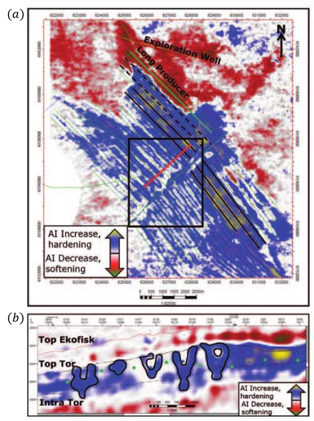
Figure 1.7: (a) Map view of inverted acoustic impedance, blue colour corresponding to AI increase/hardening and red colour representing AI decrease/softening, (b) section view showing Tor formation: blue halo shows water sweep patterns (Calvert et al., 2014).
In Valhall, the coloured inversion on the data shows the clear signal for pressure increase (a reduction in acoustic impedance) due to re-pressurization from a newly-installed injector (shown in Corzo et al., 2009). This effect is less apparent from the 4D amplitude anomaly overlaid, as this decrease could be attributed to side lobe interference. In Ekofisk, seismic impedance inversion was used as a powerful technique in detailed reservoir characterization. It was used mainly for porosity mapping and to understand reservoir layering and diagenesis. The impedance inversion results shown in Figure 1.8 reveal detailed stratigraphic facies (EL3 facies, SEE, SED2 facies, tight layer and porous layers) in Ekofisk, based on the strength of impedance (Guilbot et al., 2002).
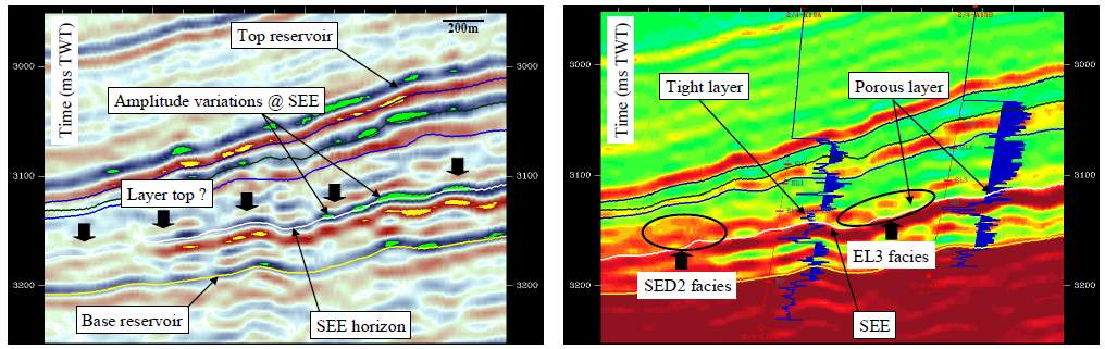
Figure 1.8: (left) Cross-section of amplitude and (right) acoustic impedance inverted from post-stack inversion – good agreement was found with log data (Guilbot et al., 2002).
In the Dan field, impedance inversion was carried out using Bayesian classification constrained by well data and rock physics analysis to define lithological boundaries and fluid distribution. The inverted products shown in Figure 1.9 illustrate the gas cap and tilted fluid contact are highlighted, where the both
IP
, and
VP
/
VS
are low. This process also helps in updating the interpretation of the top structure (Herbet et al., 2013).
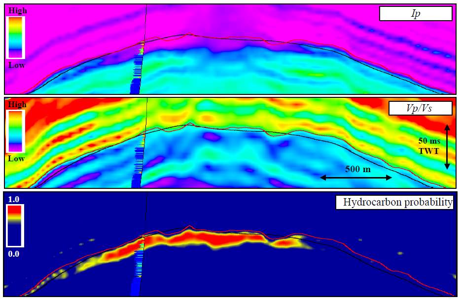
Figure 1.9: (top) Inverted acoustic impedance, (middle) inverted
VP/VS
ratio and (c) hydrocarbon probability for the Dan field (Herbet et al., 2013).
1.4 Pressure-Saturation Estimation using 4D Seismic on Chalk reservoirs
The quantification of pressure and saturation distribution is an important improvement in the interpretation and applicability of time-lapse seismic analysis, and the separation of pressure-related and saturation-related influences on the seismic response is the Holy Grail of 4D seismic. In the case of a compacting reservoir, estimation of porosity and stress changes is also top on the list of deliverables from 4D seismic. Saturation changes supply information on fluid movement and barriers, while pressure changes provide data on the position of barriers and compartments, fault sealing and non-sealing, and general connectivity. An accurate estimation of pressure and saturation requires a careful time-lapse analysis and a more quantitative integration between the engineering and seismic domains. This can be carried out by relating the changes in the seismic to corresponding changes in fluid pressure and/or saturation. The workflow presented in Figure 1.10 shows how seismic is incorporated into reservoir models: information can be compared in three key domains: seismic trace, impedance or elastic properties and the dynamic properties domain.
Different studies have shown that the matching in the seismic domain is very difficult (Gosselin et al., 2003, and Roggero et al., 2007). This is related to the nature of seismic data, which are very different from production data. Furthermore, seismic modelling is often a time intensive process. Due to CPU time constraints, reservoir simulation often requires upscaling. Thus the resolution of the simulated seismic attributes can be very low in comparison to the resolution of the observed seismic. This creates unfavourable comparisons.
Matching in the impedance or elastic property domain has its pluses and minuses. The drawbacks are that acoustic impedances are derived from a preliminary inversion process of the seismic data which is generally noisy. In addition, the result of the inversion process is largely dependent on the choice of the prior model, and thus is uncertain. However, if the seismic data is of reasonable quality, the inverted acoustic impedance, which is an interval property, proves to be an attribute that can be compared to the predicted ones more effectively. The petro-elastic model, which is key in this process, requires many calibrations from well logs and laboratory stress sensitivity coefficients and assumptions (Landrø, 2001, Gosselin et al., 2003, Stephen et al., 2005, Floricich, 2006, Wen et al., 2006, Amini, 2014).
The third domain is to compare maps or volumes of the dynamic properties such as pressure and saturation changes, inverted from seismic, which can be directly compared to the outputs of the simulation model prediction; this helps to reduce ambiguity in interpretation. However, these inverted products carry more uncertainties than elastic changes. If pressure and saturation changes can be accurately and effectively extracted from time-lapse seismic data, a direct comparison can be made with predictions from the engineering domain. There have been other methods that circumvent the complex seismic modelling process to arrive at these dynamic properties, which will be provided in Section 1.5.
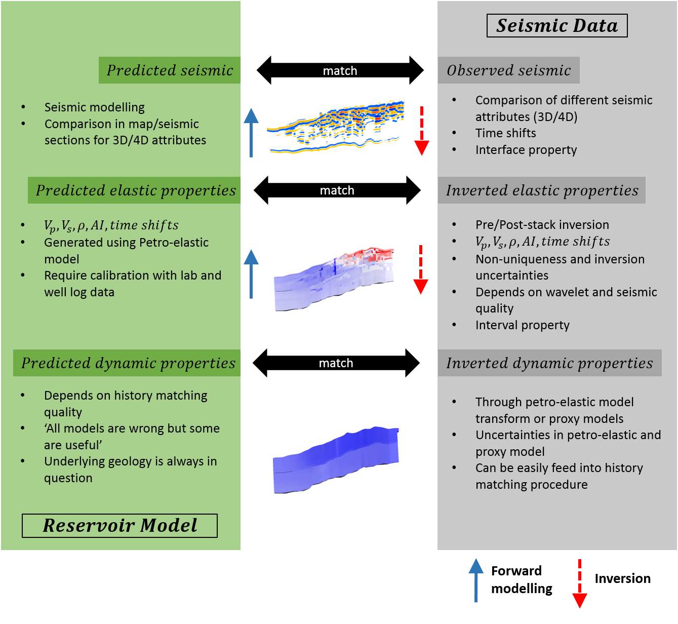
Figure 1.10: A workflow showing how to make a comparison of the seismic data to the reservoir model (engineering domain). Comparisons can be carried out in the domains of seismic, elastic properties and dynamic properties
The majority of pressure -saturation inversion work reported in the literature is mainly focused on the development and application of model driven approaches. In these methods, dynamic properties are inverted using AVO inversion which is based on the physical principles of seismic wave propagation. It is often a two-step procedure, where seismic amplitudes are inverted into various elastic properties and, subsequently, using a rock physics transform, these elastic properties are translated into pressure and saturation changes. In the work of Herwanger et al. (2010), angle-band stacks of baseline and monitor surveys are used as inputs to invert for acoustic impedance and Poisson’s ratio and the ratio changes of these parameters. A calibrated rock physics model then allows translation of these elastic properties into pressure, water saturation and porosity changes. The results from this deterministic 4D AVO inversion work are reported in Figure 1.11. In general, model-driven approaches are computation-intensive and could be hard to parameterise.
Data-driven methods, on the other hand, use production and seismic data at well locations to compute some correlations. The correlations established at these sample points are then used to estimate pressure and saturation changes from 4D seismic at the un-sampled locations between wells. In data-driven approaches, pressure-saturation estimation is driven by what is learned from field data, and thus sometimes does not require a rock-physics model. Further examples will be given in Section 1.5. In the current literature, most data-driven 4D seismic inversion commonly results in 2D maps displaying changes in reservoir pressure and saturation. This represents a major shortcoming of the approach when compared to model-driven methods that generate 3D volumetric changes in reservoir pressure and saturation. Extending the data-driven method into volumetric or into 3D space is one of the goals of this thesis. I will also discuss the rationale of breaking way from 2D maps for the Ekofisk field in Section 1.5.
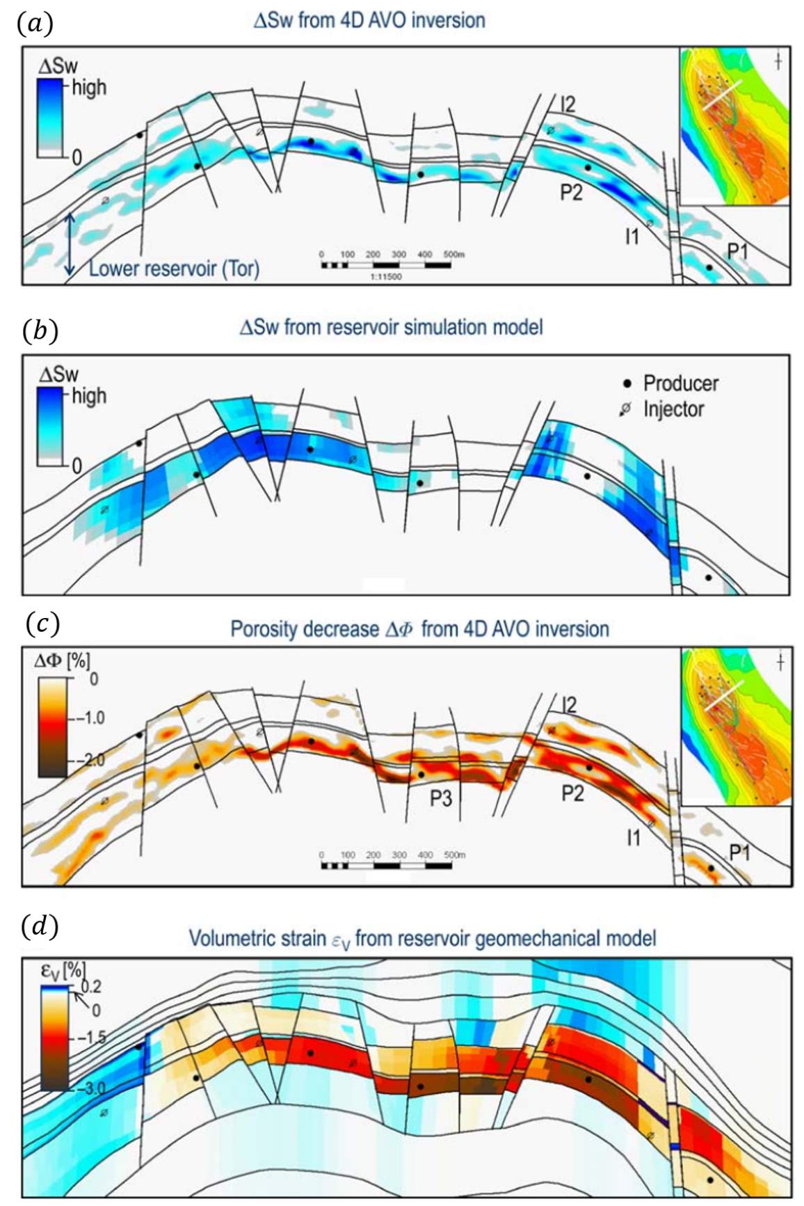
Figure 1.11: (a) Water saturation change inverted from 4D AVO inversion compared to (b) water saturation predicted from reservoir simulation model. (c) and (d) show comparisons for porosity changes from an inversion result and volumetric strain from a geomechanical model (Herwanger et al, 2010).
1.4.1 Taking advantage of multiple repeated surveys
The move towards more quantitative interpretation requires analysis of multiple 4D seismic attributes to estimate the engineering measures of reservoir change. According to Watts (2011), the use of seabed mounted four-component receiver technology will bring 4D seismic data to whole new level of data quality, with an unprecedented level of repeatability and multi-azimuth sampling of seismic wave field. Therefore, dedicated PRM data could provide an important contribution in this area of development. Well engineers in the Valhall Field have been some of the most enthusiastic customers of PRM data (Caldwell et al., 2015). The current state of the industry, as highlighted in the red box in Figure 1.12, shows how seabed systems have provided a significant step-change in reservoir monitoring. Field operation and management decisions are taken on a monthly to weekly basis, where PRM data can effectively provide new snapshots of the reservoir in that time frame.
There are many examples showing the benefits of repeated surveys and a permanent reservoir monitoring (PRM) system. One of such examples is the Clair field, as illustrated in Figure 1.13, showing a towed streamer data in 1992, a sparse OBC in 2002 and lastly the high-density OBC from 2006 to present day. What is being demonstrated is a significant improvement in data quality from a narrow azimuth acquisition to full, coarsely-sampled data, to well-sampled full azimuth data (Davies et al., 2011). It can be seen that there is a step change in improving the structural imaging and low frequency of the data.
Hypothetically, if changes in the dynamic properties of the reservoir can be easily and effectively inverted from multiple seismic data across different time periods, this could ultimately replace the concept of a simulation model. Building an up-scaled geological model (simulation model) requires a tremendous amount of time, effort and data. Moreover, the constrained reservoir models obtained by history matching with well production data often yield solutions that are not unique, and data is sparse and local. In the Ekofisk field, with dedicated PRM surveys, seismic data are acquired and processed as often as every six months (Bertrand et al., 2014). This provides a unique opportunity to monitor these reservoirs and retrieve information from the subsurface at an unprecedented pace, often surpassing the time required to history match the entire simulation model from start to finish.
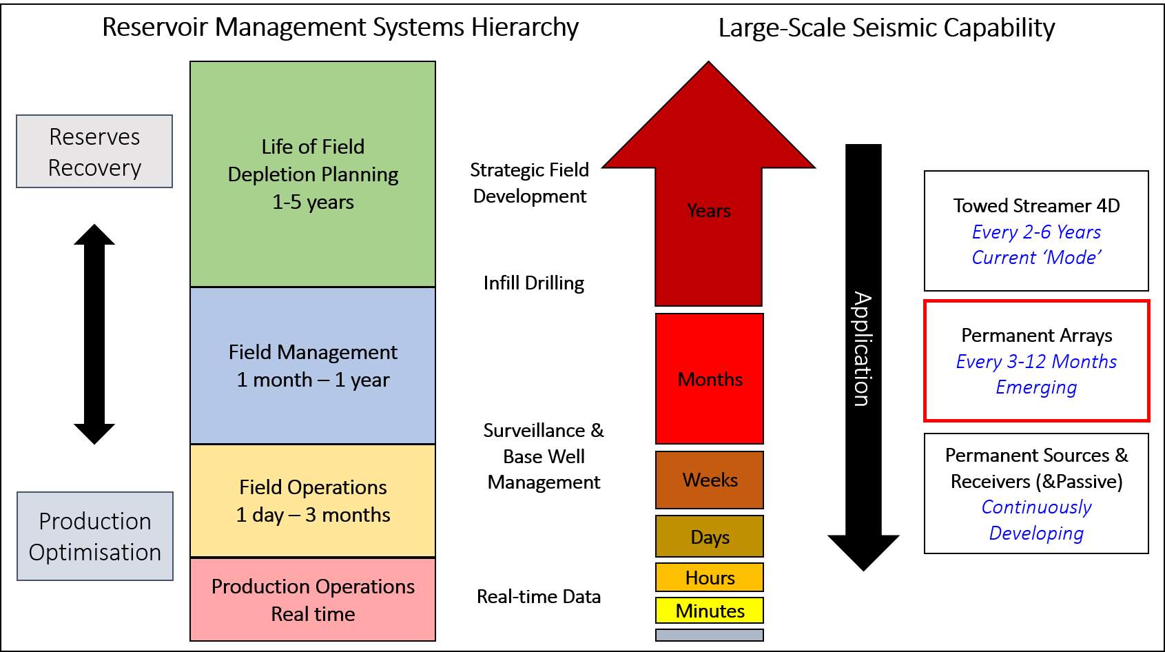
Figure 1.12: Many oil management decisions and interventions are made on a monthly basis. This could benefit from input from more frequently acquired seismic data (highlighted in red box) than is the current norm (Reproduced after Caldwell et al., 2015).
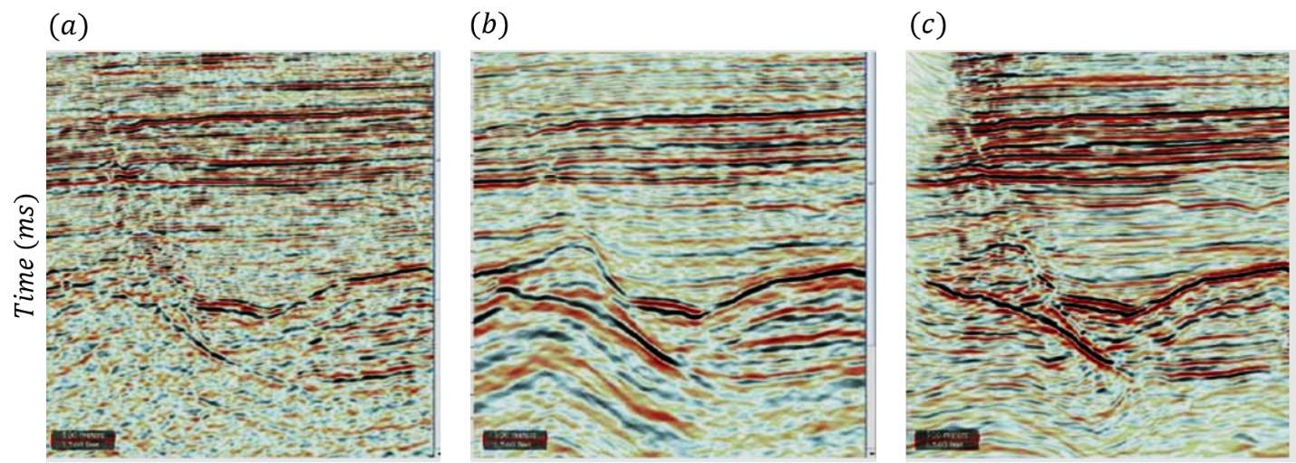
Figure 1.13: A comparison of seismic quality for (a) a towed streamer, (b) sparse OBC, and (c) high-density OBC (taken from Davies et al., 2011).
1.5 A Proxy Model Solution
One branch of active research is the determination of quantitative estimates of pressure and saturation changes from observed 4D seismic signals. Myriad techniques have been developed over the years, and these fall between two end-members – those based on rock-physics models, such as Tura and Lumley (1999), Cole et al. (2002), Landrø et al. (2003), Davolio et al. (2011) and Trani et al. (2011), and those relying on statistical calibration against the well or field wide production data, such as Landrø (2001), MacBeth et al. (2004), Floricich et al. (2006), Chu and Gist (2010), and Falahat et al. (2013). The major challenge with all these methods is that one needs to ensure that a forward model can adequately describe time-lapse elastic properties as a function of the dynamic reservoir parameters, and that the inverted dynamic properties are realistic and engineering consistent (EC).
1.5.1 Rationale of a Proxy Model approach
The use of a proxy model for inversion, modelling and production optimization is becoming more popular. For example, MacBeth et al. (2004, 2006) proposed an approach for inversion of pressure and saturation changes, where the linear relationship in Equation 1.1 describes the change of pressure and oil saturation with time-lapse seismic attributes.
∆Ax,yA̅b≈Cs∆Sox,y+Cp∆P(x,y)
(1.1)
The constants
Cs
and
Cp
can be determined by calibration against production data for wells or the simulation model. The change in time-lapse amplitude difference is normalized by the amplitude computed in the baseline survey. Multiple seismic attributes can be used and the above linear system is to be solved in the least-squares sense, to invert for pressure changes and saturation changes (Floricich et al., 2006). Such a linear relationship is said to be generally valid for a petroleum reservoir under production. Work from Alvarez and MacBeth (2013) shows that Equation 1.1 can also be written as Equation 1.2:
∆A=Cs∆Sw-Cp∆P
(1.2)
where the controlling parameters
Cs
and
Cp
provide the balance between the relative contribution of saturation and pressure change to the overall time-lapsed seismic signature. The negative sign in Equation 1.2 shows that an increase in water saturation (hardening of impedance) has an opposing physical effect on the reservoir, to an increase in pore pressure (softening of impedance), when
Cs
and
Cp
are both positive values.
The key trends that shape my proposed equation come from Floricich et al. (2006) and Corzo et al. (2013), where 4D seismic attributes are directly calibrated against field production data, and with the latter, a linear relationship was found between porosity, pressure changes and 4D amplitude changes in the compacting Valhall field. Linearity is not a necessary condition for this type of approach, as in the presence of complicated rock deformation mechanisms like water weakening, non-linear compaction trends can also be captured in the forward modelling procedure and subsequently used for inversion. In the work of Corzo et al. (2013), initial porosity was included to solve for pressure changes, specifically pressure depletion:
∆A=C1φi+C2∆P (1.3)
where C1 and C2 are fixed constants to be determined for a particular reservoir. Initial porosity,
φi
was considered as an important factor in inverting for pressure depletion in the Valhall field, a different mechanical stress sensitivity characteristics, depending on whether the initial porosity is above or below 35%. A higher initial porosity gives rise to stronger stress sensitivity, whilst lower porosity rocks are less stress sensitive for similar pressure ranges. This is similarly to the case of Ekofisk, where different mechanical stress sensitivity is found above and below 28% of initial porosity. The relationship between the time-lapse attribute (speed-up) versus pressure depletion as a function of initial porosity is shown in Figure 1.14 (a) and (b). The results of the inversion applied on the Valhall field are shown in Figure 1.15. The general conclusion from this work is that the estimation of pressure depletion from time-lapse seismic differs from the simulation model in some areas and the approach is easily implemented and data-driven.
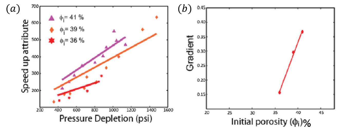
Figure 1.14: (a) Correlation between speed-up attribute from 4D seismic and pressure depletion from pressure change predicted from simulation model at well perforations and (b) the variation of the resultant gradient term (C1) with initial porosity (Corzo et al., 2013).
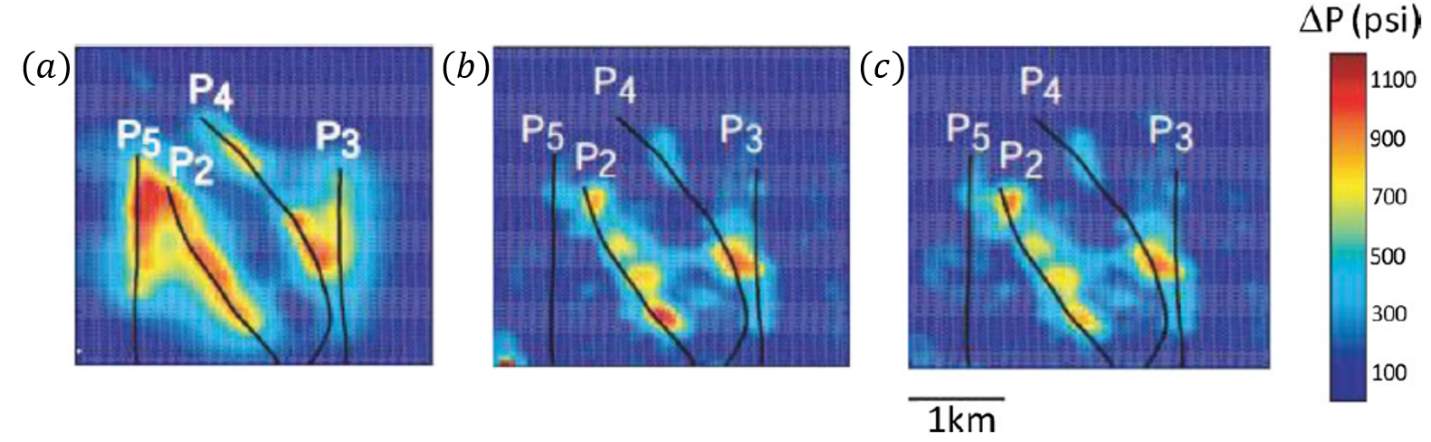
Figure 1.15: Estimated pressure change from (a) a coupled geomechanical-fluid flow simulator, (b) inverted using 4D seismic amplitude attribute – Largest Positive Value (LPV) with initial porosity averaged from certain layers in the reservoir and (c) inverted from LPV using initial porosity of one zone only (Corzo et al., 2013).
This technique is also employed by Landa et al. (2015), where the correlation between 4D seismic and pressure-saturation information is obtained by calibrating with well data. Uncertainty or probabilistic analysis in the map-based estimation of reservoir pressure and saturation changes is performed in the calibration process in order to bring forward the uncertainty in this process to the final estimation of pressure and saturation changes. These uncertainties include seismic noise, location of top and bottom surfaces to compute seismic attributes, and the production data. The pressure and saturation changes estimated for a clastic turbidite reservoir are presented in Figure 1.16.
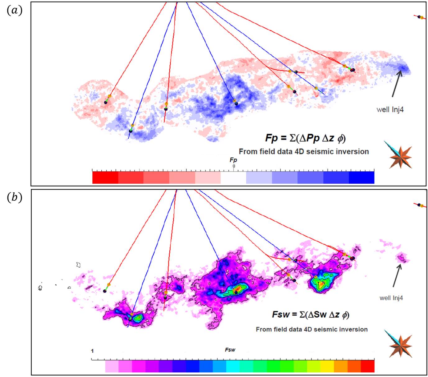
Figure 1.16: (a) Maps of inverted pressure change and (b) water saturation change from Landa et al., (2015) using a data-driven inversion approach.
I am inspired to break away from the map-based approach into something more suitable for the thick, multi-cycle, compacting chalk reservoir of the Ekofisk field. Equation 1.3 applied in the Valhall field is not totally applicable to Ekofisk, due to their different production history and the nature of the reservoirs, such as their heterogeneity and thickness. Ekofisk had twenty-nine years of water injection between 1987 and 2015, whereas the water flooding in Valhall has only been operating for nine years, to date, and full scale water injection only started in 2007. This implies the water weakening signal is less dominant in the Valhall field in comparison to Ekofisk. The map-based approach of Equation 1.3 works effectively in Valhall, since the main producing Tor formation is only 30m thick, which translates to half a cycle on the seismic data (Jack et al., 2010). A comparative study between Valhall and Ekofisk is provided in Table 1.1, highlighting the main differences between the two neighbouring chalk fields:
| Ekofisk | Valhall | |
| Thickness | Ekofisk formation (100 to 168 metres), Tight Zone (20m on average), Tor formation (76 to 152 metres)
Multicycles |
Tor is on average 30m, Hod is thicker but only contributes 8% to production
Half cycle |
| Burial depth | 2896 – 3261 m | 2400 m |
| Water weakening behaviour |
|
|
| Production history | Production in 1971
Full field water injection In 1987 (after 17 years of primary depletion) |
Production in 1982
Water injection in 2007 (after 26 years) 20 years on primary depletion |
Table 1.1: Showing a comparison between Valhall and Ekofisk in terms of reservoir thickness, burial depth, geomechanical behaviour and production history.
1.5.2 Proxy models in other applications
The concept of a proxy model is novel in the oil and gas related disciplines, but it has a long and pivotal history in the fields of optimisation, statistics and uncertainty quantification. A proxy model is used to provide a fast approximation to the actual function (Goodwin, 2015). Some of the proxy models used in the oil and gas industry include the surrogate model, the kriging model, neural networks, and the regression model. In history matching, response surface proxies are commonly used to approximate the functional relationship between the input parameters and the aggregated mismatch (Castellini et al., 2006, Friedmann et al., 2003, Landa and Güyagüler, 2003). The mismatch function in history matching is the misfit between the simulated data and observed data (Tarantola, 2005), which quantifies the degree of consistency of a reservoir model and the historical data. Each evaluation of the mismatch function requires a simulation run, making the history matching process laborious and computationally expensive. One way to reduce the computational cost is to construct a response surface proxy for the mismatch function, which is a parameterized mathematical expression that can be calibrated on a set of training data to approximate the input to output relations of the mismatch function. After calibration, the response surface proxy can be used to replace the simulator to evaluate the mismatch function.
Other uses of proxy include using an analytical expression to speed up the estimation of seismic data using outputs from the reservoir simulator instead of running a full simulator-to-seismic workflow. As successfully demonstrated by Fursov (2015), a linear relationship between seismic and reservoir dynamic properties: pressure, water and gas saturation change:
∆A=ap∆P+aSw∆Sw+aSg∆Sg∙A0 (1.4)
was used to generate seismic attributes to speed up the history matching process.
A0 is the seismic attribute at baseline survey. The coefficients ap, aSw and aSg
in the equation are calculated from seismic data of the given reservoir from multiplemonitors. The left hand side of the equation will include all the points of time-lapse attribute maps from all monitors; the right hand side will include the points of the reservoir dynamic property maps from the corresponding time steps, scaled by the baseline seismic attribute. According to the findings obtained by Fursov (2015), the fast-track procedures, conducted by applying a regression between 4D seismic attribute maps and the average maps of the dynamic reservoir properties, are considerably faster than the full-fledged history matching. However, the fast track method is more applicable if noise is low, whereas the slower history matching workflows are more robust for the situation where there are noisier inputs.
Map vs. volume
Thin and thick reservoirs should be treated differently for interpretation. Because many of the sand thickness in clastic reservoirs are below tuning thickness, many case studies on 4D amplitude interpretation employ a quadrature-phase difference approach (Johnston, 2013). Moreover, for a thin reservoir, quadrature amplitude analysis is useful if the reservoir is a half cycle, such as in the North Sea clastic Schiehallion field. In that case, changes in amplitude are then directly related to the primary changes in impedance. Map-based methods will be sufficient, since averaging across a thin reservoir will not compromise the signal too much. In contrast, thick reservoirs will have a very different character at both top and base of the reservoir; thus, when looking at maps, this reservoir should be interpreted using top and base maps separately and with caution, instead of averaging the amplitude difference across the entire reservoir thickness.
The caveats of interpreting such reservoirs are interference, tuning and side lobe problems. The 4D signals will comprise of too many destructive and constructive events and will not truly reflect primary changes, such as in the case of the Ekofisk field. This is also one of the reasons that prompts us to look at volumes instead of maps. Moreover, this is particularly true for long wavelength spatial components such as pressure; averaging the time-lapse response across the entire reservoir will smear the signal significantly if there is a competing response between pressure and saturation. Imagine there is a pressure gradient from top to base of the reservoir: computing a single map for the entire reservoir will significantly underestimate the actual magnitude and spatial distribution of the signal. Table 1.2 shows the common analysis carried out for both thin and thick reservoirs, the caveats are associated with the reservoir thickness, the effectiveness of the interpretation and the necessity of a volume based approach. In this thesis, I will demonstrate a new method to invert for changes in pressure and saturation for a thick and multicycle reservoir such as the Ekofisk field, in three dimensions.
| Reservoir type | Analysis | Caveats | Interpretation | 2D versus 3D |
| Thin | Quadrature amplitude analysis |
|
Reflects primary impedance changes |
|
| Thick |
|
|
Does not reflect primary reservoir dynamic changes |
|
Table 1.2: Showing a compilation of the type of analysis, caveats of those analysis, methods of interpretation and 2D versus 3D interpretation on thin versus thick reservoirs.
1.6 Focus of this Thesis
1.6.1 Outline of the thesis
This thesis will develop the ideas of monitoring changes inside the reservoir, namely changes in dynamic properties, such as pressure and saturation changes, by utilizing time-lapse seismic observations from both inside and outside the reservoir. Chapters 4 and 5 focus on using time-lapse seismic attributes inside the reservoir, whereas Chapters 6 and 7 utilise overburden time-lapse anomalies induced by production changes.
Here are the contents of the remaining seven chapters of my thesis, in brief:
Chapter 2 provides an overview of the literature on the Ekofisk field, covering topics from geological setting to field production history and the challenges in geomechanics. I also evaluate various rock physics models to establish a suitable rock physics model for the Ekofisk field. This rock physics model is calibrated using data from rock mechanics, well logs and mineral moduli from the literature.
Chapter 3 shows how 4D seismic data are used for dynamic reservoir characterization in the Ekofisk field. A summary of the seismic data from both acquisition strategies, streamer and Life of Field Seismic (LoFS) is provided. An analysis is carried out to compare and contrast the reservoir time-shifts in both types of surveys and the correlation with different production mechanisms.
Chapter 4 presents the formulation of a new equation to invert for pressure and saturation changes in a thick, compacting chalk reservoir. A synthetic model is created to understand the impact of rock compaction and different dynamic changes on impedance changes. By employing backward engineering, the composite impedance change is decomposed to analyse its individual components and workings in detail, in order to recreate the same property using a proxy model. Physical phenomena such as water weakening and compaction, which are notorious in chalk reservoirs, are accounted for in the proxy model, and also described in this chapter.
Chapter 5 applies the proxy model set out in Chapter 4 to data from the Ekofisk field, in the Norwegian North Sea. A stochastic approach via Bayesian McMC is employed to invert for the changes in pressure and saturation and to capture uncertainties in the result.
Chapter 6 shows a different route to estimate pressure changes by using time-lapse information from the overburden. The Geertsma pressure inversion method from Hodgson (2009) provides the basis for a linear inversion scheme to estimate both pressure changes and also the Hatchell-Bourne-RØste R-factor. A synthetic example is provided to demonstrate the success of estimating the R-factor by constraining the inversion result with pressure information from a well-history matched simulation model.
Chapter 7 applies the inversion scheme introduced in Chapter 6 to the Ekofisk field. This chapter draws conclusions on the average R-factor recovered in the Ekofisk field. The chapter also discuss the R-factors calculated for different regions of pressure build-up and drawdown identified in the field, and the results confirm the current understanding determined by laboratory experiments and previous studies that the magnitude varies as a function of strain polarity, with the asymmetry being at most a factor of three.
Chapter 8 presents a summary of the thesis. In addition, recommendations are also made for further development of the ideas presented in this thesis.
1.6.2 Publications
Parts of this thesis have been independently presented in the following publication:
Wong, M. Y., MacBeth, C., JafarGandomi, A., Bertrand, A., and Amini, H. (2017). An Engineering-consistent approach for separating pressure and saturation changes in the Ekofisk field. Petroleum Geoscience. (Accepted with revision)
1.6.3 Conferences with extended abstracts
Wong M. Y., MacBeth, C., and Amini, H. (2017). Time-shifts Interpretation of legacy and frequent repeat seismic data in a compacting chalk reservoir. 79th EAGE Conference and Exhibition.
Wong, M.Y., and MacBeth, C. (2016). R-factor Recovery via Geertsma’s Pressure Inversion Assisted by Engineering Concepts. EAGE Geophysics and Geomechanics, Jointly Applied to Subsurface Characterisation workshop.
Wong, M.Y., JafarGandomi, A., MacBeth C., and Bertrand, A. (2015). Pressure and saturation change inversion using 4D seismic: Application to a chalk reservoir in North Sea, SEG International Exposition and Annual Meeting.
Wong, M.Y., MacBeth, C., and Bertrand, A. (2015). Engineering Consistent Constraints for the Inversion of Changes in Pressure and Saturation on Ekofisk.77th EAGE Conference and Exhibition.
Wong, M.Y., MacBeth, C., and Bertrand, A. (2015). Engineering Consistent Constraints for the Inversion of Changes in Pressure and Saturation on Ekofisk. EAGE 4D Workshop: Getting the most out of 4D – from reservoir to surface.
Cite This Work
To export a reference to this article please select a referencing stye below:
Related Services
View all


Related Content
All TagsContent relating to: "Engineering"
Engineering is the application of scientific principles and mathematics to designing and building of structures, such as bridges or buildings, roads, machines etc. and includes a range of specialised fields.
Related Articles

DMCA / Removal Request
If you are the original writer of this dissertation and no longer wish to have your work published on the UKDiss.com website then please: